2. model Package¶

This package provides two kinds of models:

Generative pointprocess models (see Section ni.model.pointproccess)

GLM based inhomogeneous pointprocess (ip) models

The pointprocess models can instantiate a given firing rate function with a spike train. The ip models use “components” that are combined to fit a spike train using a GLM.

2.1. What is a “component”?¶

For the ni.model package, a component is a set of time series (or a way to generate these) in a Generalized Linear Model that is used to fit a set of spike trains. When a model is fitted to a set of spike trains, the components are used to compute the designmatrix. Each component provides 1 or more timeseries that represent the influence of a specific event or aspect that is expected to affect the firing rate at that specific point in time to a certain degree.

Eg. a component can be as simple as a constant value over time, or it can be 0 for most of the time, except at those time points where a specific event occurs (eg. a spike of a different neuron). The design matrix shown here is mostly 0 and contains three components (history, rate and a constant):

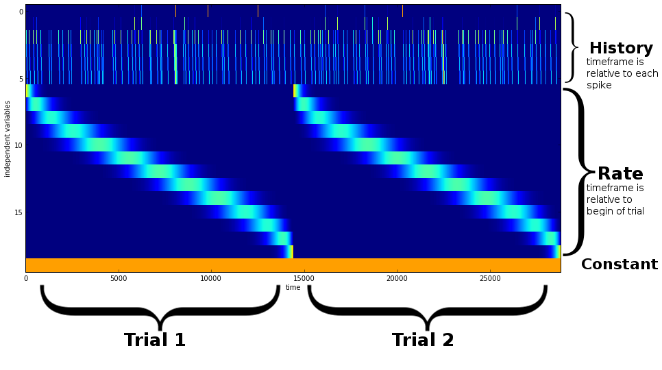
To model a more or less precise time course of the effect of an event, the component needs to create mutiple time series, each representing a time window relative to the event (usually following the event, if a causal link is assumed). It is convenient to use splines to model these windows, because they will produce a smooth time series when summed. These time windows can be arranged linearly (each spanning the same amount of time) or logarithmically (such that there is a higher resolution close to the event than further away). The length and number of the time windows can be adjusted, since their explanatory value depends on the modeled process.

2.2. The Rate component¶

Given that each spike train is alligned in the same timeframe regarding a certain stimulus (or sequence of stimuli), a rate component models rate fluctuations that occur in every trial. This is done by creating a number of timeseries, each representing a portion of the trial time: eg. early in the trial, in the middle of the trial, at the end of the trial.

A ni.model.designmatrix.RateComponent will span the whole trial with a given number of knots while the class ni.model.designmatrix.AdaptiveRateComponent will use the firing rate to space out the knots to cover (on average) an equal amount of spikes.

2.3. The history components¶

Since the spike data containers contain multiple spike trains, a component can access the spiketimes of each of the spike trains contained. The history components use these spike times to model the effect of a certain spike train on the dependent spike train.

autohistory: the effect of the spike train on itself. Eg. refractory period or periodic spiking

crosshistory: models the effect of another spike train on the one modeled

2nd order autohistory_2d: for bursting neurons, the autohistory alone will not capture the behaviour of the neuron, as it has to either predict periodic activity for the whole trial or no auto effect at all. The 2nd order history takes into account two spikes, such that the end of a burst can be predicted.

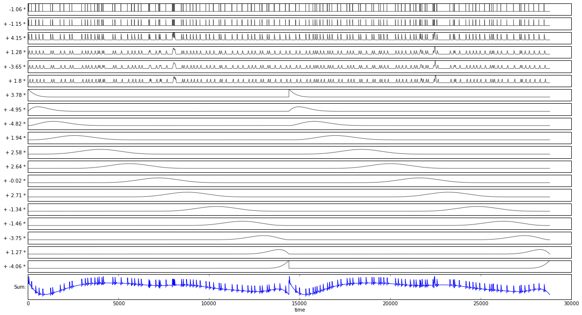
Here you can see the slow time frame of a rate fluctuation (fixed to the time frame of each trial) and the fast time frame of a history component (each relative to a spike):

2.4. Configuring a Model¶

The model class has a default behaviour that assumes you want to have one rate component, one autohistory componenet and a crosshistory component for each channel. This behaviour can be changed by providing a different configuration dictionary to the model.

Eg. to create a model without any of the components:

model = ni.model.ip.Model({‘name’:’Model’,’autohistory’:False, ‘crosshistory’:False, 'rate':False})

Or, if additionally the 2nd order autohistory should be enabled:

model = ni.model.ip.Model({‘name’:’Model’,’autohistory_2d’:True })

Important for models is also which spike train channel should be modeled by the others:

model_0 = ni.mode.ip.Model({'cell':0})
model_1 = ni.mode.ip.Model({'cell':1})
model_2 = ni.mode.ip.Model({'cell':2})
model_3 = ni.mode.ip.Model({'cell':3})

Instead of only true or false, crosshistory can also be a list of channels that should be used:

model = ni.mode.ip.Model({'cell':1,'crosshistory':[2]}) # cell 1 modeled using activity of cell 2

Also there are a number of configuration options that are passed on to a component to change its behaviour:

Rate Component:

knots_rate: how many knots should be created

adaptive_rate: Whether the RateComponent or AdaptiveRateComponent should be used. The AdaptiveRateComponent can additionally be tweaked with:

adaptive_rate_exponent (default = 2)

adaptive_rate_smooth_width (default = 20)

History Components (autohistory and crosshistory):

history_length: total lenght of the time spanned by the history component

history_knots: number of knots to span

These options are set for the whole model at once:

model = ni.mode.ip.Model({'knots_rate':10,'history_length':200}) # sets history_length for autohistory and crosshistory, knots_rate for rate component

2.5. Fitting a Model¶

An ip.Model can be fitted on a ni.data.data.Data object and will produce a ni.model.ip.FittedModel. This will contain the fitted coefficients and the design templates, such that the different components can be inspected individually:

model = ni.model.ip.Model({'cell':2,'crosshistory':[1,3]})
fm = model.fit(data.trial(range(data.nr_trials/2)))

fm.plot_prototypes() # will plot each fitted component

plot(fm.firing_rate_model().sum(1)) # will plot the firing rate components (rate + constant)

plot(fm.statistics['pvalues']) # plots the pvalues for each coefficient

2.6. Creating custom components¶

To be precise, what happens when a model is fitted is the following:

The model creates a ni.model.designmatrix.DesignMatrixTemplate and adds components (which are subclasses of ni.model.designmatrix.Component) according to its configuration to it:

when the Component classes are created they are provided with most of the information they need (eg. trial length)

The DesignMatrixTemplate is combined with the data which creates the actual designmatrix by:

For each component the function getSplines is called, providing the component with spikes of other neurons

The component returns a 2 dimensional numpy array that has the dimensions of length of time x number of time series

if the array does not have the length of the complete time series, it will be repeated until it fits. So a kernel that has the length of exactly one trial will be repeated for each trial (the ni models by default make all trials the same length).

The design matrix is then passed to the GLM fitting backend

So, if you want to add a component, this can be either implement a function getSplines that returns a 2d numpy array that has the correct dimensions (time bins x N), or you can use or inherit from ni.model.designmatrix.Component and set the self.kernel attribute which will then be returned:

my_kernel = ni.model.create_splines.create_splines_linspace(time_length, 6, 0) # creates a 6 knotted set of splines covering time_length
c = Component(header='My own component',kernel=my_kernel)
model = ni.model.ip.Model(custom_components = [c])

Applications can be eg. a rate component that is only applied to trials, while a second component is applied to the others. If two kinds of trials are alternated this could be done like this:

from ni.model.designmatrix import Component
my_kernel = ni.model.create_splines.create_splines_linspace(time_length, 6, 0) # creates a 6 knotted set of splines covering time_length
is_trial_type_1 = repeat([0,1]*(number_of_trials/2),trial_length)
is_trial_type_2 = 1 - is_trial_type_1
c1 = Component(header='Trial Type 1 Rate',kernel=np.concatenate([my_kernel]*number_of_trials) * is_trial_type_1[:,np.newaxis])
c2 = Component(header='Trial Type 2 Rate',kernel=np.concatenate([my_kernel]*number_of_trials) * is_trial_type_2[:,np.newaxis])
model = ni.model.ip.Model({'custom_components': [c1,c2]},trial_length)

Or alternatively you can overwrite a kernel of the rate component:

kernel = np.concatenate([
            np.concatenate([my_kernel]*number_of_trials) * is_trial_type_1[:,np.newaxis]),
            np.concatenate([my_kernel]*number_of_trials) * is_trial_type_2[:,np.newaxis])
        ])
model = ni.model.RateModel({’rate’:True, ’custom_kernels’: [{’Name’:’rate’,’Kernel’: kernel}]})

2.7. Classes in the ni.model package¶

class ni.model.BareModel(configuration={})[source]¶

Bases: ni.model.ip.Model

This is a shorthand class for an Inhomogenous Pointprocess model that contains no Components.

This is completely equivalent to using:

ni.model.ip.Model({‘name’:’Bare Model’,’autohistory’:False, ‘crosshistory’:False, ‘rate’:False})

class ni.model.RateModel(knots_rate=10)[source]¶

Bases: ni.model.ip.Model

This is a shorthand class for an Inhomogenous Pointprocess model that contains only a RateComponent and nothing else.

This is completely equivalent to using:

ni.model.ip.Model({‘name’:’Rate Model’,’autohistory’:False, ‘crosshistory’:False, ‘knots_rate’:knots_rate})

class ni.model.RateAndHistoryModel(knots_rate=10, history_length=100, history_knots=4)[source]¶

Bases: ni.model.ip.Model

This is a shorthand class for an Inhomogenous Pointprocess model that contains only a RateComponent, a Autohistory Component and nothing else.

This is completely equivalent to using:

ni.model.ip.Model({‘name’:’Rate Model with Autohistory Component’,’autohistory’:True, ‘crosshistory’:False, ‘knots_rate’:knots_rate, ‘history_length’:history_length, ‘knot_number’:history_knots})

2.7.1. `ip` Module¶

class ni.model.ip.Configuration(c=False)[source]¶

Bases: ni.tools.pickler.Picklable

The following values are the defaults used:

name = “Inhomogeneous Point Process”

cell = 0

Which cell to model in the data (index)

Boolean Flags for Default Model components (True: included, Fals: not included):
autohistory = True
crosshistory = True
rate = True
constant = True
autohistory_2d = False
backend = “glm”

The backend used. Valid options: “glm” and “elasticnet”

backend_config = False

knots_rate = 10

Number of knots in the rate component

adaptive_rate = False
Whether to use linear spaced knots or an adaptive knot spacing, which depends on the variability of the firing rate. Uses these two options:
adaptive_rate_exponent = 2
adaptive_rate_smooth_width = 20
history_length = 100

Length of the history kernel

knot_number = 3

Number of knots in the history kernel

custom_kernels = []
List of kernels that overwrite default component behaviour. To overwrite the rate component use:
[{ 'Name':'rate', 'Kernel': np.ones(100) }]
custom_components = []

List of components that get added to the default ones.

self.be_memory_efficient = True

Whether or not to save the data and designmatrix created by the fitting model

Unimportant options no one will want to change:
delete_last_spline = True 
design = 'new'
mask = np.array([True])
Look at the [source] for a full list of defaults.

class ni.model.ip.FittedModel(model)[source]¶

Bases: ni.tools.pickler.Picklable

When initialized via Model.fit() it contains a copy of the configuration, a link to the model it was fitted from and fitting parameters:

FittedModel. fit

modelFit Output

FittedModel. design

The DesignMatrix used. Use design.matrix for the actual matrix or design.get(‘...’) to extract only the rows that correspond to a keyword.

compare(data)[source]¶

Using the model this will predict a firing probability function according to a design matrix.

Returns:

Deviance_all: dv, LogLikelihood_all: ll, Deviance: dv/nr_trials, LogLikelihood: ll/nr_trials, llf: Likelihood function over time ll: np.sum(ll)/nr_trials

complexity[source]¶: returns the length of the parameter vector

dumps()[source]¶: see ni.tools.pickler

family_fitted_function(p)[source]¶: only implemented family: Binomial

firing_rate_model()[source]¶: returns a time series which contains the rate and constant component

generate(bins=-1)[source]¶

Generates new spike trains from the extracted staistics

This function only uses rate model and autohistory. For crosshistory dependence, use ip_generator.

bins

How many bins should be generated (should be multiples of trial_length)

getParams()[source]¶: returns the parameters of each design matrix component as a list

getPvalues()[source]¶: returns pvalues of each component as a dictionary

html_view()[source]¶: see ni.tools.html_view

plotParams(x=-1)[source]¶: plots the parameters and returns a dictionary of figures

plot_firing_rate_model()[source]¶: returns a time series which contains the rate and constant component

plot_prototypes()[source]¶: plots each of the components as a prototype (sum of fitted b-splines) and returns a dictionary of figures

predict(data)[source]¶: Using the model this will predict a firing probability function according to a design matrix.

prototypes()[source]¶: returns a dictionary with a prototype (numpy.ndarray) per component

pvalues_by_component()[source]¶: returns pvalues of each component as a dictionary

class ni.model.ip.Model(configuration=None, nr_bins=0)[source]¶

Bases: ni.tools.pickler.Picklable

backend[source]¶

cell[source]¶

compare(data, p, nr_trials=1)[source]¶

will compare a timeseries of probabilities p to a binary timeseries or Data instance data.

Returns:

Deviance_all: dv, LogLikelihood_all: ll, Deviance: dv/nr_trials, LogLikelihood: ll/nr_trials, llf: Likelihood function over time ll: np.sum(ll)/nr_trials

dm(in_spikes, design=None)[source]¶: Creates a design matrix from data and self.design

in_spikes ni.data.data.Data instance

design (optional) a different designmatrix.DesignMatrixTemplate

fit(data=None, beta=None, x=None, dm=None, nr_trials=None)[source]¶

Fits the model

in_spikes ni.data.data.Data instance

example:

from scipy.ndimage import gaussian_filter
import ni
model = ni.model.ip.Model(ni.model.ip.Configuration({'crosshistory':False}))
data = ni.data.monkey.Data()
data = data.condition(0).trial(range(int(data.nr_trials/2)))
dm = model.dm(data)
x = model.x(data)
from sklearn import linear_model
betas = []
fm = model.fit(data)
betas.append(fm.beta)
print "fitted."
for clf in [linear_model.LinearRegression(), linear_model.RidgeCV(alphas=[0.1, 1.0, 10.0])]:
        clf.fit(dm,x)
        betas.append(clf.coef_)

        figure()
        plot(clf.coef_.transpose(),'.')
        title('coefficients')
        prediction = np.dot(dm,clf.coef_.transpose())
        figure()
        plot(prediction)
        title('prediction')
        ll = x * log(prediction) + (len(x)-x)*log(1-prediction)
        figure()
        plot(ll)
        title('ll')
        print np.sum(ll)

fit_with_design_matrix(fittedmodel, spike_train_all_trial, dm)[source]¶: internal function

generateDesignMatrix(data, trial_length)[source]¶: generates a design matrix template. Uses meta data from data to determine number of trials and trial length.

html_view()[source]¶: see ni.tools.html_view

predict(beta, data)[source]¶: will predict a firing probability function according to a design matrix.

x(in_spikes)[source]¶: converts data into a dependent variable time series, ie. it chooses the cell that was configured and extracts only this timeseries.

2.7.2. `designmatrix` Module¶

class ni.model.designmatrix.AdaptiveRateComponent(header='rate', rate=False, exponent=2, knots=10, length=1000, kernel=False)[source]¶

Bases: ni.model.designmatrix.Component

Rate Design Matrix Component

header: name of the kernel component rate: a rate function that determines exponent: the rate function will be taken to thins power to have a higher selctivity for high firing rates knots: Number of knots length: length of the component. Will be multiplied

kernel: use this kernel instead of a newly created one

getSplines(data=[])[source]¶

class ni.model.designmatrix.Component(header='Undefined', kernel=0)[source]¶

Bases: ni.tools.pickler.Picklable

Design Matrix Component

header: name of the kernel component kernel: kernel that will be tiled to fill the design matrix

getSplines(data=[])[source]¶

class ni.model.designmatrix.DesignMatrix(length, width=1)[source]¶

Bases: ni.tools.pickler.Picklable

Use DesignMatrixTemplate to create a design matrix.

This class computes an actual matrix, where DesignMatrixTemplate can be saved before the matrix is instanciated.

add(splines, header)[source]¶

addLinSpline(knots, header, length=0)[source]¶

addLogSpline(knots, header, length=0)[source]¶

clip()[source]¶

get(filt)[source]¶

getIndex(filt)[source]¶

getMask(filt)[source]¶

plot(filt='')[source]¶

setMask(mask)[source]¶

class ni.model.designmatrix.DesignMatrixTemplate(length, trial_length=0)[source]¶

Bases: ni.tools.pickler.Picklable

Most important class for Design Matrices

Uses components that are then combined into an actual design matrix:

>>> DesignMatrixTemplate(data.nr_trials * data.time_bins)
>>> kernel = cs.create_splines_logspace(self.configuration.history_length, self.configuration.knot_number, 0)
>>> design_template.add(designmatrix.HistoryComponent('autohistory', kernel=kernel))
>>> design_template.add(designmatrix.HistoryComponent('crosshistory'+str(2), channel=2, kernel = kernel))
>>> design_template.add(designmatrix.RateComponent('rate',self.configuration.knots_rate,trial_length))
>>> design_template.add(designmatrix.Component('constant',np.ones((1,1))))
>>> design_template.combine(data)

add(component)[source]¶: Adds a component

combine(data)[source]¶

combines the design matrix template into an actual design matrix.

It needs an ni.Data instance for this to place the history splines.

get(filt)[source]¶: returns the splines of the first component, the header of which matches filt

getIndex(filt)[source]¶: returns the index (design matrix rows) of the component matching filt

getMask(filt)[source]¶: reurns the mask of the component matching filt

get_components(filt)[source]¶: returns all component, the header of which matches filt

setMask(mask)[source]¶: sets a mask (list of boolean values), which design matrix rows to use. Default is all True. If mask is shorter` than the desgin matrix, all following values are assumed True.

class ni.model.designmatrix.HistoryComponent(header='autohistory', channel=0, history_length=100, knot_number=4, order_flag=1, kernel=False, delete_last_spline=True)[source]¶

Bases: ni.model.designmatrix.Component

History Design Matrix Component

Will be convolved with spikes before fitting

header: name of the kernel component channel: which channel the kernel should be convolved with (default 0) history_length: length of the kernel knot_number: number of knots (will be logspaced) order_flag: default 0 (no higher order interactions)

kernel: use this kernel instead of a newly created one

Atm only order 1 interactions

getSplines(channels=[])[source]¶

class ni.model.designmatrix.HistoryDesignMatrix(spikes, history_length=100, knot_number=5, order_flag=1, kernel=False)[source]¶: Internal helper class

class ni.model.designmatrix.RateComponent(header='rate', knots=10, length=1000, kernel=False)[source]¶

Bases: ni.model.designmatrix.Component

Rate Design Matrix Component

header: name of the kernel component knots: Number of knots length: length of the component. Will be multiplied

kernel: use this kernel instead of a newly created one

getSplines(data=[])[source]¶

class ni.model.designmatrix.SecondOrderHistoryComponent(header='autohistory', channel_1=0, channel_2=0, history_length=100, knot_number=4, order_flag=1, kernel_1=False, kernel_2=False, delete_last_spline=True)[source]¶

Bases: ni.model.designmatrix.Component

History Design Matrix Component with Second Order Kernels

Will be convolved with spikes before fitting

header: name of the kernel component channel: which channel the kernel should be convolved with (default 0) history_length: length of the kernel knot_number: number of knots (will be logspaced) order_flag: default 0 (no higher order interactions)

kernel: use this kernel instead of a newly created one

Atm only order 1 interactions

getSplines(channels=, []get_1d_splines=False, beta=False)[source]¶

ni.model.designmatrix.convolve_spikes(spikes, kernel)[source]¶: Convolves a spike train with a kernel by adding the kernel onto every spiketime.

ni.model.designmatrix.convolve_spikes_2d(spikes_a, spikes_b, kernel_a, kernel_b)[source]¶: Does a 2d convolution

2.7.3. `net_sim` Module¶

The Net Simulator is divided into a Configuration, Net and a Result object.

After configuration of the network it can be instantiated by calling Net(conf) with a valid configuration conf. This creates eg. random connectivity so that the simulation with the same network can be repeated multiple times.

c = ni.model.net_sim.SimulationConfiguration()
c.Nneur = 10
net = ni.model.net_sim.Net(c)
print net
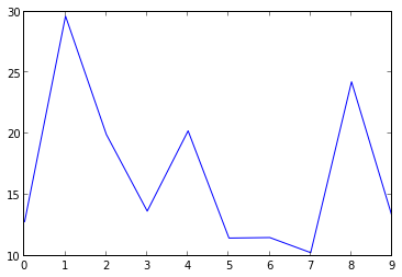
net.plot_firing_rates()

'ni.model.net_sim' Simulation Setup
Timerange: (250, 10250)
 10 channels with firing rates: 
        [12.815928361, 29.6328550796, 19.9415819867, 13.6710936491, 20.242131795, 11.4661487294, 11.5071338947, 10.2727521514, 24.2587596858, 13.1497981307]
Firing Rates plot

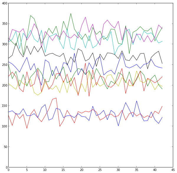
for i in range(1,11):
    print i
    res1 = net.simulate()
    res1.plot_firing_rates()

plot(numpy.array([r.num_spikes_per_channel for r in net.results]))
plot([0]*len(net.results))

class ni.model.net_sim.Net(config)[source]¶

The Net Simulator class. Use with an Configuration instance.

load(filename)[source]¶: loads itself from a file

plot_firing_rates()[source]¶: plots the intended firing rates

plot_interaction()[source]¶: plots the interactions of the network

save(filename)[source]¶: saves itself to a file

simulate()[source]¶: Simulates the network

class ni.model.net_sim.SimulationConfiguration[source]¶

Configures the simulation. The default values are:

Nneur = 100 sparse_coeff = 0.1 Trial_Time = 1000 prior_epoch = 250 Ntrials = 10 Nsec = Ntrials*Trial_Time/1000 Ntime = Nsec*1000 eps =0.1 frate_mu = 1.0/25.0 Nhist = 50 output = False rate_function = False

Nsec[source]¶

Ntime[source]¶

class ni.model.net_sim.SimulationResult[source]¶

Holds the results of a simulation

data[source]¶

plot()[source]¶: plots the resulting spike train

plot_firing_rates()[source]¶: plots the resulting firing rate

plot_firing_rates_per_channel()[source]¶: plots the firing rate for each channel

stopTimer()[source]¶: stops the internal timer

store(data)[source]¶: stores data in the container

ni.model.net_sim.simulate(config)[source]¶: creates a network and simulates it.

2.7.4. `create_design_matrix_vk` Module¶

ni.model.create_design_matrix_vk.computeCovariate(index, o, C, V1)[source]¶: Computes a row of the designMatrix corresponding to a certain covariate.

ni.model.create_design_matrix_vk.create_design_matrix_vk(V1, o)[source]¶

Fills free rows in the current design matrix, deduced from size(mD) and len(freeCov), corresponding to a single covariate according to the spline bases of Volterra kernels. The current kernel(s) and the respective numbers of covariates that will be computed for each kernel is deduced from masterIndex by determining the position in hypothetical upper triangular part of hypercube with number of dimensions corresponding to current kernel order. Using only the ‘upper triangular part’ of the hypercube reflects the symmetry of the kernels which stems from the fact that only a single spline is used as basis function.

saves covariate information in cell array ‘covariates’, format is {kernelOrder relativePositionInKernel productTermsOfV1}

Anpassung für Gordon: masterIndex, log, C, mD, freeCov werden berechnet statt übergeben.

ni.model.create_design_matrix_vk.detKernels(freeCov, masterIndex, oCov, mOrder, C)[source]¶: Determines from the number of free slots in Designmatrix len(freeCov) and the current masterIndex how many covariates for which Volterra coefficient can be computed. Updates model order mOrder.

ni.model.create_design_matrix_vk.detModelOrder(masterIndex, C)[source]¶: Determines model order and corresponding number of covariates.

ni.model.create_design_matrix_vk.numCov(C, complexity)[source]¶: Computes number of covariates in a model for which len(complexity) symmetric kernels are assumed.

ni.model.create_design_matrix_vk.upTriHalf(C, cDim)[source]¶: Computes number of elements in upper triangular half of hybercube.

2.7.5. `create_splines` Module¶

ni.model.create_splines.N(u, i, p, knots)[source]¶

Compute Spline Basis

Evaluates the spline basis of order p defined by knots at knot i and point u.

ni.model.create_splines.augknt(knots, order)[source]¶: Augment knot sequence such that some boundary conditions are met.

ni.model.create_splines.create_splines(length, nr_knots, remove_last_spline, fn_knots)[source]¶: Generates B-spline basis functions based on the length and number of knots of the ongoing iteration. fn_knots is a function that computes the knots.

ni.model.create_splines.create_splines_linspace(length, nr_knots, remove_last_spline)[source]¶: Generates B-spline basis functions based on the length and number of knots of the ongoing iteration

ni.model.create_splines.create_splines_logspace(length, nr_knots, remove_last_spline)[source]¶: Generates B-spline basis functions based on the length and number of knots of the ongoing iteration

ni.model.create_splines.spcol(x, knots, spline_order)[source]¶

Computes the spline colocation matrix for knots in x.

The spline collocation matrix contains all m-p-1 bases defined by knots. Specifically it contains the ith basis in the ith column.

Input:

x: vector to evaluate the bases on knots: vector of knots spline_order: order of the spline

Output:

colmat: m x m-p matrix: The colocation matrix has size m x m-p where m denotes the number of points the basis is evaluated on and p is the spline order. The colums contain the ith basis of knots evaluated on x.

ni.model.create_splines.spline(x, knots, p, i=0.0)[source]¶: Evaluates the ith spline basis given by knots on points in x

2.7.6. `backend_elasticnet` Module¶

This module provides a backend to the .ip model. It wraps the sklearn.linear_model.ElasticNet / ElasticNetCV objects.

class ni.model.backend_elasticnet.Configuration[source]¶

Default Values:

crossvalidation = True

If true, alpha and l1_ratio will be calculated by crossvalidation.

alpha = 0.5

l1_ratio = 1

be_memory_efficient = True

Does not keep the data with which it is fitted.

class ni.model.backend_elasticnet.Fit(f, m)[source]¶

predict(X=False)[source]¶

class ni.model.backend_elasticnet.Model(c=False)[source]¶

fit(x, dm)[source]¶

ni.model.backend_elasticnet.compare(x, p, nr_trials=1)[source]¶

ni.model.backend_elasticnet.predict(x, dm)[source]¶

2.7.7. `backend_glm` Module¶

This module provides a backend to the .ip model. It wraps the statsmodels.api.GLM object.

class ni.model.backend_glm.Configuration[source]¶

Default Values:

be_memory_efficient = True

Does not keep the data with which it is fitted.

class ni.model.backend_glm.Fit(f, m)[source]¶

predict(X=False)[source]¶

class ni.model.backend_glm.Model(c=False)[source]¶

fit(y, X)[source]¶

ni.model.backend_glm.compare(x, p, nr_trials=1)[source]¶

ni.model.backend_glm.predict(x, dm)[source]¶

ni 0.2 documentation

2. model Package

2. model Package¶

2.1. What is a “component”?¶

2.2. The Rate component¶

2.3. The history components¶

2.4. Configuring a Model¶

2.5. Fitting a Model¶

2.6. Creating custom components¶

2.7. Classes in the ni.model package¶

2.7.1. ip Module¶

2.7.2. designmatrix Module¶

2.7.3. net_sim Module¶

2.7.4. create_design_matrix_vk Module¶

2.7.5. create_splines Module¶

2.7.6. backend_elasticnet Module¶

2.7.7. backend_glm Module¶

2.7.1. `ip` Module¶

2.7.2. `designmatrix` Module¶

2.7.3. `net_sim` Module¶

2.7.4. `create_design_matrix_vk` Module¶

2.7.5. `create_splines` Module¶

2.7.6. `backend_elasticnet` Module¶

2.7.7. `backend_glm` Module¶