Usage
Running a model
>>> import convis
>>> retina = convis.retina.Retina()
>>> retina(some_short_input)
>>> retina.run(some_input,dt=100)
Usually PyTorch Layers are callable and will perform their forward computation when called with some input. But since Convis deals with long (potentially infinite) video sequences, a longer input can be processed in smaller chunks by calling Layer.run(input,dt=..) with dt set to the length of input that should be processed at a time. This length depends on the memory available in your system and also if you are using the model on your cpu or gpu.
run() also accepts numpy arrays as input, which will be converted into PyTorch Tensor`s and packaged as a `Variable.
Input and Output
The in- and output of convis models is in most cases five-dimensional. Why is that?
The convention comes from Conv3d processing two additional dimensions for 3d convolutions: batches and channels. They are handled differently in the way they relate to the convolution weight: each batch is processed completely independently and adding more batches does not require a change to the weight and there are always the same number of output as input batches; in turn each channel (eg. colour) requires an appropriate in_channel dimension in the weight and the number of output channels is also determined by the dimensions of the weight (see convis.filters.Conv3d).
The dimensions of all output in convis is therefore:
[batch, channel, time, space x, space y]
and the Output objects can also contain multiple output tensors of different shapes.
>>> o = retina.run(some_input,dt=100)
>>> print(o[0].size())
torch.Size([1, 1, 1000, 10, 10])
>>> print(o[1].size()) # the retina model has by default two outputs (On and Off cells)
torch.Size([1, 1, 1000, 10, 10])
If an input has less dimensions, it can be broadcasted with convis.make_input() from 1d, 2d and 3d to 5d, and this function also gives the option to create CPU or GPU tensors. Also 3d inputs will be automatically broadcast to 5d by all convis.base.Layer s.
How to Plot
To get an overview plot of an Output object in jupyter notebooks, it is sufficient to have the output as the last line in a cell.
This will call convis.plot_tensor() on each tensor in the Output.
Alternatively one can call convis.base.Output.plot(), which will get a line plot of the first tensor (or the n-th tensor if an argument n is supplied).
In [1]: o = retina.run(some_input,dt=100)
        o
Out[1]: Output containing 2 Tensors.

        | 1x1x1000x1x1 Tensor
        | <line plot>
        | <sequence of example frames>

        | 1x1x1000x1x1 Tensor
        | <line plot>
        | <sequence of example frames>

In [2]: o.plot(0)
Out[2]: <line plot>

In [3]: convis.plot(o[0])
Out[3]: <line plot (same as o.plot())>

In [4]: convis.plot_tensor(o[0])
Out[4]: <line plot>
        <sequence of example frames>
Most analysis will be done on numpy.array() s on the CPU rather than torch.Tensor s, so the output can be turned into arrays with the function convis.base.Output.array():
>>> out = o.array(0) # using first tensor in output
>>> out
array([[[[[0,0,0,0,0,0,0,0,0]],
        ... ]]], dtype=uint8)
>>> plot(out[0,0,:,5,5])     # signal of pixel 5,5 over time
>>> imshow(out[0,0,100,:,:]) # frame at time 100
If there is more than one tensor in the Output object, o.array(1) will give the second output, etc.
Animating Plots
Another way to plot 5d tensors if you are using jupyter notebooks is to produce an animation. Convis offers two animation functions (plain and scrolling) with two outputs each (html5 video and html/javascript animation):
>>> convis.animate_to_html(o.array(),skip=5,scrolling_plot=True,window_length=500) # html and scrolling
<HTML+javascript animated plot>
>>> convis.animate_to_video(o.array(),skip=5,scrolling_plot=False) # video and plain
<HTML5 embedded video>
The output can also be produced manually from the animate()
and animate_double_plot() functions, which each return
a matplotlib.animation.FuncAnimation:
>>> from IPython.display import HTML
>>> HTML(convis.variable_describe.animate(o.array(),skip=10).to_html5_video())
<HTML5 embedded video>
>>> HTML(convis.variable_describe.animate_double_plot(o.array(),skip=10,window_length=500).to_jshtml())
<HTML+javascript animated plot>
Or you can save the animation (see matplotlib.animation.FuncAnimation.save()):
>>> convis.variable_describe.animate(o.array(),skip=10).save('mymovie.mp4')
>>> convis.variable_describe.animate_double_plot(o.array(),skip=10,window_length=500).save('mymovie.mp4')
Global configurations
There are a few global parameters that can change the behaviour of convis. They can be found by tab completing convis.default_(…).
To enable or disable whether Parameters should by default keep their computational graph you can set convis.default_grad_enabled to either True or False. If you are not planning on using the optimization features of convis, you can disable all computational graphs to save memory! By default, graphs are enabled (convis.default_grad_enabled = True).
import convis
convis.default_grad_enabled = False # disables computational graphs by default
convis has default scaling parameters for spatial and temporal dimensions.
import convis
# 20 pixel correspond to 1 degree of the visual field
convis.default_resolution.pixel_per_degree = 20
# a bin is by default 1 ms long
convis.default_resolution.steps_per_second = 1000

# making all computations faster, but less accurate:
convis.default_resolution.pixel_per_degree = 10  # spatial scale is half the default
convis.default_resolution.steps_per_second = 200 # 5ms time bins
Configuring a Model: the .p. parameter list
The best way to configure the model is by exploring the
structure with tab completion of the .p. parameter list.
As an example. the retina model will give you first the list of layers and
then the list of parameters of each layer (see also convis.base.Layer).
To change the values, you can use the method .set, or (but only if you use the `.p.` list) by assigning a new value to the parameter directly:
>>> retina = convis.retina.Retina()
>>> retina.p.<tab>
opl, bipolar, gang_0_input, gang_0_spikes, gang_1_input, gang_1_spikes
>>> retina.p.bipolar.lambda_amp
Variable
----------
   name: lambda_amp
   doc: Amplification of the gain control. When `lambda_amp`=0, there is no gain control.
   value: array([0.], dtype=float32)
>>> retina.p.bipolar.lambda_amp.set(100.0)
>>> retina.p.bipolar.lambda_amp = 100.0
>>> retina.p.bipolar.lambda_amp
Variable
----------
   name: lambda_amp
   doc: Amplification of the gain control. When `lambda_amp`=0, there is no gain control.
   value: array([100.], dtype=float32)
The .p list is collecting all the parameters of the model, so that they are easier for you to interact with. You can also navigate through the submodules yourself, but then you have to ignore all methods and attributes of the Layers that are not Parameters:
>>> retina.bipolar.<tab>
a_0, a_0, a_1, a_1, add_module, apply, b_0, b_0, children, clear_state, compute_loss, conv2d, cpu, cuda, dims, dims, double, dump_patches, eval, float, forward, g_leak, g_leak, g_leak, get_all, get_parameters, get_state, half, init_states, inputNernst_inhibition, inputNernst_inhibition, input_amp, input_amp, input_amp, lambda_amp, lambda_amp, lambda_amp, load_parameters, load_state_dict, m, modules, named_children, named_modules, named_parameters, optimize, p, parameters, parse_config, plot_impulse, plot_impulse_space, pop_all, pop_optimizer, pop_parameters, pop_state, preceding_V_bip, preceding_attenuationMap, preceding_inhibition, push_all, push_optimizer, push_parameters, push_state, register_backward_hook, register_buffer, register_forward_hook, register_forward_pre_hook, register_parameter, register_state, retrieve_all, run, s, save_parameters, set_all, set_optimizer, set_optimizer, set_parameters, set_state, share_memory, state_dict, steps, steps, store_all, tau, tau, tau, train, training, training, type, user_parameters, zero_grad
>>> # too many!
>>> retina.bipolar.lambda_amp
Variable
----------
   name: lambda_amp
   doc: Amplification of the gain control. When `lambda_amp`=0, there is no gain control.
   value: array([0.], dtype=float32)
>>> retina.bipolar.lambda_amp.set(42.0)
Since retina.bipolar is itself a convis.base.Layer object, retina.bipolar.p.<tab>
works the same as retina.p.bipolar.<tab>.
Note
In the following case the Parameter object will be replaced by the number 100.0. It will no longer be optimizable or exportable:
>>> retina.bipolar.lambda_amp = 100.0 # <- .p is missing!
Instead you can use .set() to set the value, or replace the Parameter with a new Parameter:
>>> retina.bipolar.lambda_amp.set(100.0)
>>> retina.p.bipolar["lambda_amp"].set(100.0)
Another feature of the .p. list are the special attributes _all and _search. .p._all. gives you tab completable list without hierarchy, ie. all variables can be seen at once.
>>> retina.p._all.<tab>
gang_0_input_spatial_pooling_weight, gang_1_spikes_refr_sigma, gang_0_input_i_0, gang_1_spikes_noise_sigma, bipolar_lambda_amp, gang_1_input_sign, gang_0_input_lambda_G, gang_0_input_transient_tau_center, gang_1_spikes_refr_mu, gang_1_input_sigma_surround, gang_1_input_spatial_pooling_bias, bipolar_input_amp, gang_0_input_v_0, gang_0_spikes_tau, gang_1_input_transient_relative_weight_center, gang_1_input_transient_tau_center, bipolar_conv2d_weight, gang_0_input_sign, gang_0_spikes_refr_sigma, bipolar_g_leak, gang_0_spikes_refr_mu, gang_0_input_transient_weight, bipolar_tau, gang_1_spikes_tau, gang_1_input_f_transient, gang_0_spikes_g_L, gang_1_input_lambda_G, gang_1_spikes_g_L, gang_0_input_transient_relative_weight_center, gang_0_input_f_transient, gang_0_input_sigma_surround, gang_1_input_v_0, gang_0_spikes_noise_sigma, gang_1_input_i_0, opl_opl_filter_relative_weight, gang_1_input_transient_weight
The _search attribute can search in this list for any substring:
>>> retina.p._search.lam.<tab>
gang_1_input_lambda_G, bipolar_lambda_amp, gang_0_input_lambda_G
>>> retina.p._search.i_0.<tab>
gang_0_input_i_0, gang_1_input_i_0
Both of these can be iterated over instead of tab-completed:
>>> for p in retina.p._search.i_0:
        p.set(10.0)
>>> for name,p in retina.p._search.i_0.__iteritems():
        print(name)
        p.set(10.0)
gang_0_input_i_0
gang_1_input_i_0
Configuring a Model: exporting and importing all parameters
You can get a dictionary of all parameter values
>>> d = retina.get_parameters()
>>> d['opl_opl_filter_surround_E_tau']
array([0.004], dtype=float32)
>>> d['opl_opl_filter_surround_E_tau'][0] = 0.001
>>> retina.set_parameters(d)
Switching between CPU and GPU usage
PyTorch objects can move between GPU memory and RAM by calling .cuda() and .cpu() methods respectively. This can be done on a single Tensor or on an entire model.
Enabling and disabling the computational graph
Each Parameter has by default its requires_grad attribute set to True,
which means that every operation done with this Parameter will be recorded, so that
we can use backpropagation at some later timepoint. This can use a lot of memory,
especially in recursive filters, and you might not even need the computational graph.
To disable the graph for a single Parameter or Variable, supply the constructor with the
keyword argument requires_grad or call its requires_grad_()
method after the Parameter was created. The trailing underscore signifies that the method
will be executed in place and does not produce a copy of the variable.
import convis
p = convis.variables.Parameter(42, requires_grad=False)
# or later:
import convis
p = convis.variables.Parameter(42)
p.requires_grad_(False)
For a complete Layer, there is a helper function requires_grad_()
that will set the flag for all the contained Parameters:
import convis
m = convis.models.LN()
m.requires_grad_(False)
Globally, graphs can be disabled with the convis.default_grad_enabled variable:
import convis
convis.default_grad_enabled = False # disables computational graphs by default
Using Runner objects
Runner objects can execute a model on a fixed set of input and output streams. The execution can also happen in a separate thread:
import convis, time
import numpy as np

inp = convis.streams.RandomStream(size=(10,10),pixel_per_degree=1.0,level=100.2,mean=128.0)
out1 = convis.streams.SequenceStream(sequence=np.ones((0,10,10)), max_frames=10000)
retina = convis.retina.Retina()
runner = convis.base.Runner(retina, input = inp, output = out1)
runner.start()
time.sleep(5) # let thread run for 5 seconds or longer
plot(out1.sequence.mean((1,2)))
# some time later
runner.stop()
Optimizing a Model
One way to optimize a model is by using the set_optimizer() attribute and the optimize() method:
l = convis.models.LN()
l.set_optimizer.SGD(lr=0.001) # selects an optimizer with arguments
#l.optimize(some_inp, desired_outp) # does the optimization with the selected optimizer
A full example:
import numpy as np
import matplotlib.pylab as plt
import convis
import torch
l_goal = convis.models.LN()
k_goal = np.random.randn(5,5,5)
l_goal.conv.set_weight(k_goal)
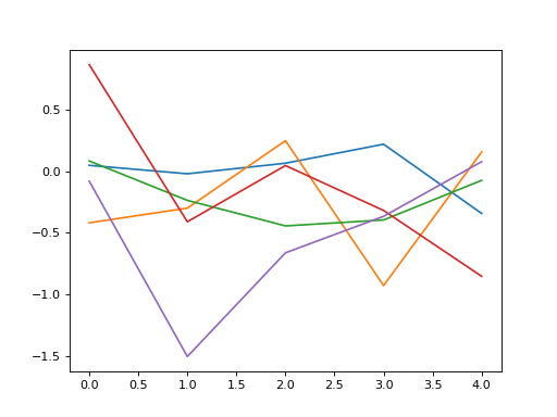
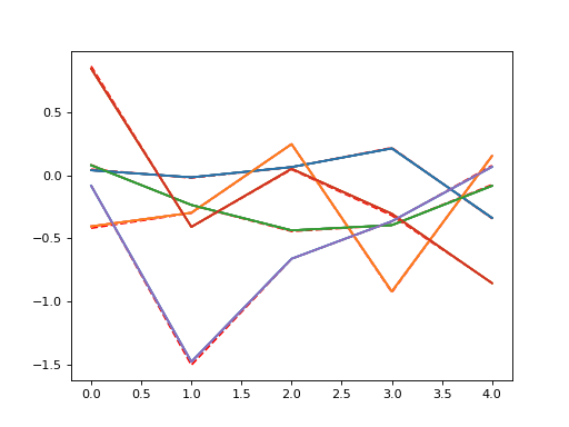
plt.plot(l_goal.conv.weight.data.cpu().numpy()[0,0,:,:,:].mean(1))
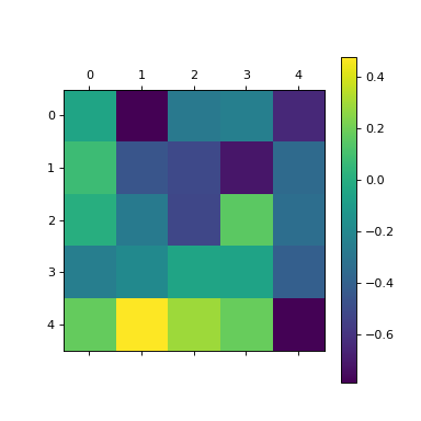
plt.matshow(l_goal.conv.weight.data.cpu().numpy().mean((0,1,2)))
plt.colorbar()
l = convis.models.LN()
l.conv.set_weight(np.ones((5,5,5)),normalize=True)
l.set_optimizer.LBFGS()
# optional conversion to GPU objects:
#l.cuda()
#l_goal.cuda()
inp = 1.0*(np.random.randn(200,10,10))
inp = torch.autograd.Variable(torch.Tensor(inp)) # .cuda() # optional: conversion to GPU object
outp = l_goal(inp[None,None,:,:,:])
plt.figure()
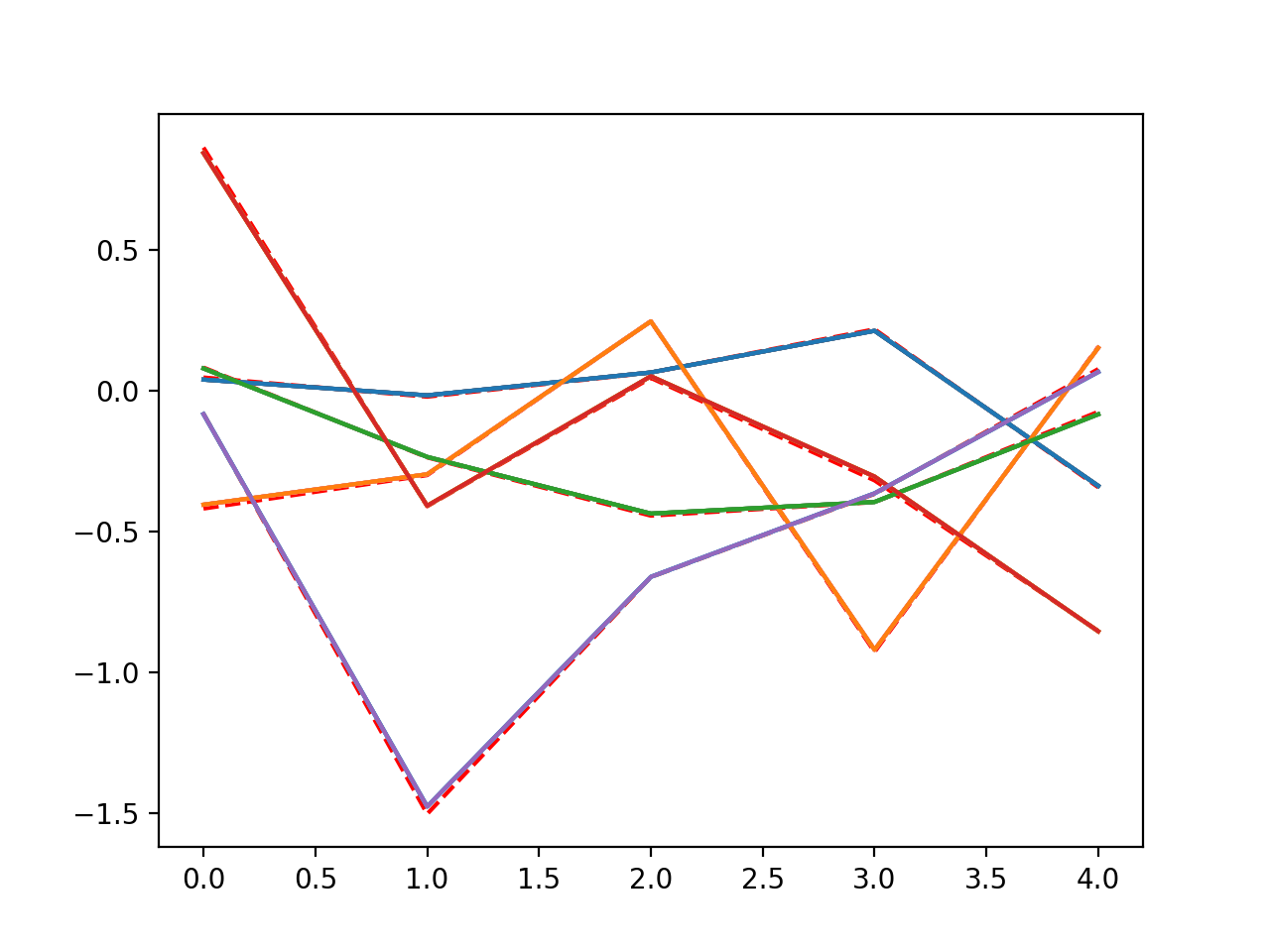
plt.plot(l_goal.conv.weight.data.cpu().numpy()[0,0,:,:,:].mean(1),'--',color='red')
for i in range(50):
l.optimize(inp[None,None,:,:,:],outp)
if i%10 == 2:
plt.plot(l.conv.weight.data.cpu().numpy()[0,0,:,:,:].mean(1))
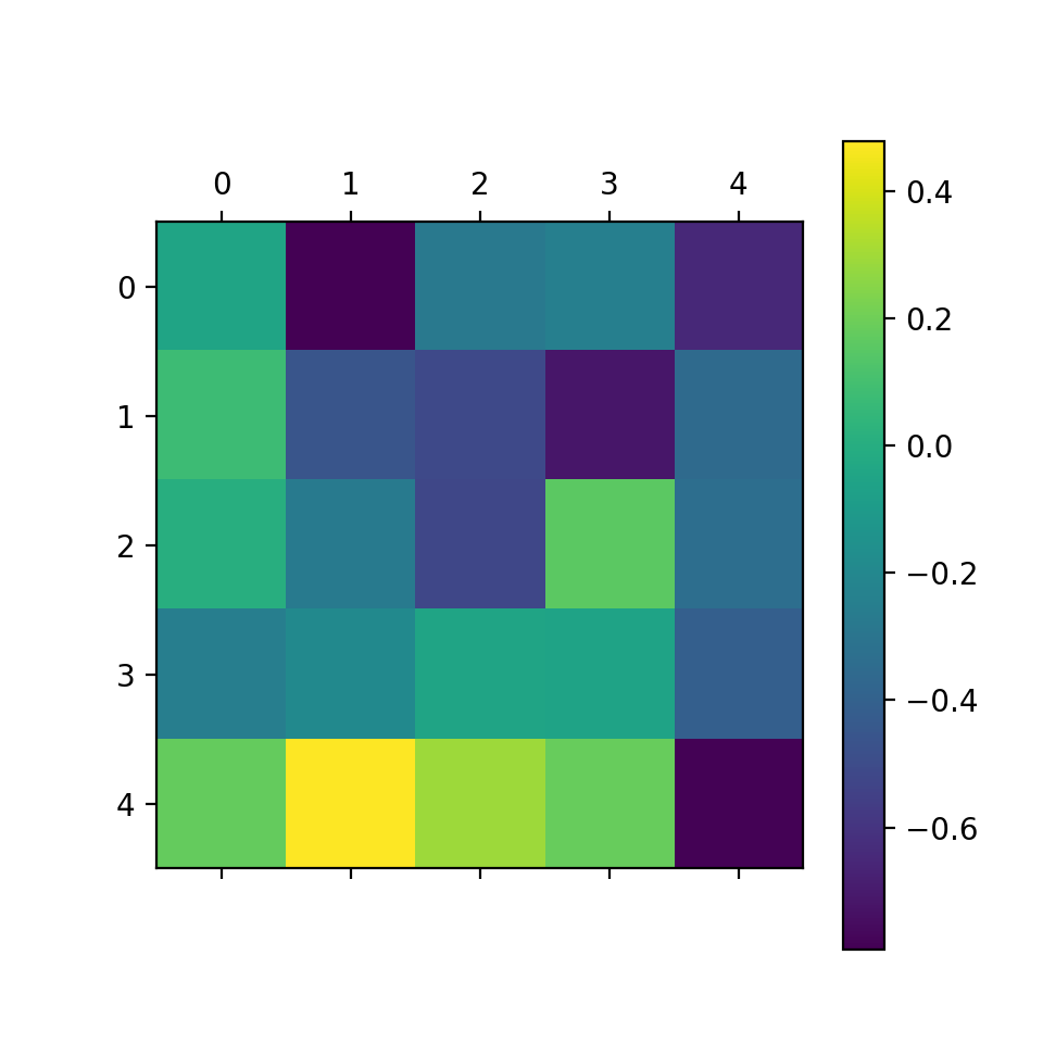
plt.matshow(l.conv.weight.data.cpu().numpy().mean((0,1,2)))
plt.colorbar()
plt.figure()
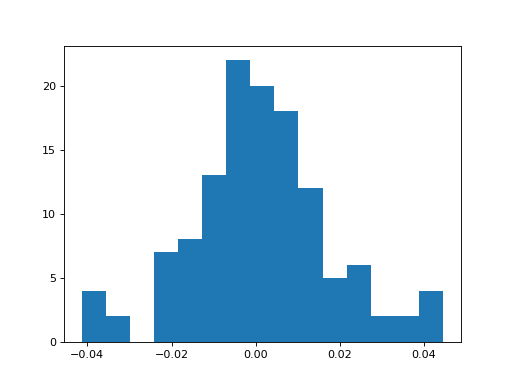
h = plt.hist((l.conv.weight-l_goal.conv.weight).data.cpu().numpy().flatten(),bins=15)


When selecting an Optimizer, the full list of available Optimizers can be seen by tab-completion.
Some interesting optimizers are:
- SGD: Stochastic Gradient Descent - one of the simplest possible methods, can also take a momentum term as an option
- Adagrad/Adadelta/Adam/etc.: Accelerated Gradient Descent methods - adapt the learning rate
- LBFGS: Broyden-Fletcher–Goldfarb-Shanno (Quasi-Newton) method - very fast for many almost linear parameters
Using an Optimizer by Hand
The normal PyTorch way to call Optimizers is to fill the gradient buffers by hand and then calling step() (see also http://pytorch.org/docs/master/optim.html ).
import numpy as np
import convis
import torch
l_goal = convis.models.LN()
k_goal = np.random.randn(5,5,5)
l_goal.conv.set_weight(k_goal)
inp = 1.0*(np.random.randn(200,10,10))
inp = torch.autograd.Variable(torch.Tensor(inp))
outp = l_goal(inp[None,None,:,:,:])
l = convis.models.LN()
l.conv.set_weight(np.ones((5,5,5)),normalize=True)
optimizer = torch.optim.SGD(l.parameters(), lr=0.01)
for i in range(50):
    # first the gradient buffer have to be set to 0
    #optimizer.zero_grad()
    # then the computation is done
    o = l(inp)
    # and some loss measure is used to compare the output to the goal
    loss = ((outp-o)**2).mean() # eg. mean square error
    # applying the backward computation fills all gradient buffers with the corresponding gradients
    #loss.backward(retain_graph=True)
    # now that the gradients have the correct values, the optimizer can perform one optimization step
    #optimizer.step()
Or using a closure function, which is necessary for advanced optimizers that need to re-evaluate the loss at different parameter values:
l = convis.models.LN()
l.conv.set_weight(np.ones((5,5,5)),normalize=True)
optimizer = torch.optim.LBFGS(lr=0.01)

def closure():
    optimizer.zero_grad()
    o = l(inp)
    loss = ((outp-o)**2).mean()
    loss.backward(retain_graph=True)
    return loss

#for i in range(50):
#    optimizer.step(closure)
The .optimize method of `convis.Layer`s does exactly the same as the code above. It is also possible to supply it with alternate optimizers and loss functions:
l = convis.models.LN()
l.conv.set_weight(np.ones((5,5,5)),normalize=True)
opt2 = torch.optim.LBFGS(l.parameters())
#l.optimize(inp[None,None,:,:,:],outp, optimizer=opt2, loss_fn = lambda x,y: (x-y).abs().sum()) # using LBFGS (without calling .set_optimizer) and another loss function
.set_optimizer.*() will automatically include all the parameters in the model, if no generator/list of parameters is used as the first argument.