Filters and Layers¶

Convolution Filters¶

covnis.filters.Conv3d is the basic 3d convolution filter and based on torch.nn.Conv3d. It can dynamically pad the input in x and y dimensions to keep the output the same size as the input. The time dimension has to be padded by another operation.

conv = covnis.filters.Conv3d(in_channels=1,out_channels=1,kernel_size=(10,20,20),bias=False,)
print(conv.weight) # the weight parameter
print(conv.bias)   # the bias parameter
conv.set_weight(np.random.rand(10,20,20),normalize=True)
some_output = conv(some_input)

Warning

Currently, the nd convolution operation can leak memory when fitting a model!

class convis.filters.Conv3d(in_channels=1, out_channels=1, kernel_size=(1, 1, 1), bias=True, *args, **kwargs)[source]¶

Does a convolution, but pads the input in time with previous input and in space by replicating the edge.

Arguments:

in_channels

out_channels

kernel_size

bias (bool)

Additional PyTorch Conv3d keyword arguments:

padding (should not be used)

stride

dilation

groups

Additional convis Conv3d keyword arguments:

time_pad: True (enables padding in time)

autopad: True (enables padding in space)

To change the weight, use the method set_weight() which also accepts numpy arguments.

set_weight(w, normalize=False, preserve_channels=False, flip=True)[source]¶

Sets a new weight for the convolution.

Parameters:

w: numpy array or PyTorch Tensor

The new kernel w should have 1,2,3 or 5 dimensions.

1 dimensions: temporal kernel 2 dimensions: spatial kernel 3 dimensions: spatio-temporal kernel (time,x,y) 5 dimensions: spatio-temporal kernels for multiple channels

(out_channels, in_channels, time, x, y)

If the new kernel has 1, 2 or 3 dimensions and preserve_channels is True, the input and output channels will be preserved and the same kernel will be applied to all channel combinations. (ie. each output channel recieves the sum of all input channels). This makes sense if the kernel is further optimized, otherwise, the same effect can be achieved with a single input and output channel more effectively.

normalize: bool (default: False)

Whether or not the sum of the kernel values should be normalized to 1, such that the sum over all input values and all output values is the approximately same.

preserve_channels: bool (default: False)

Whether or not to copy smaller kernels to all input-output channel combinations.

flip: bool (default: True)

If True, the weight will be flipped, so that it corresponds 1:1 to patterns it matches (ie. 0,0,0 is the first frame, top left pixel) and the impulse response will be exactly w. If False, the weight will not be flipped.

New in version 0.6.4.

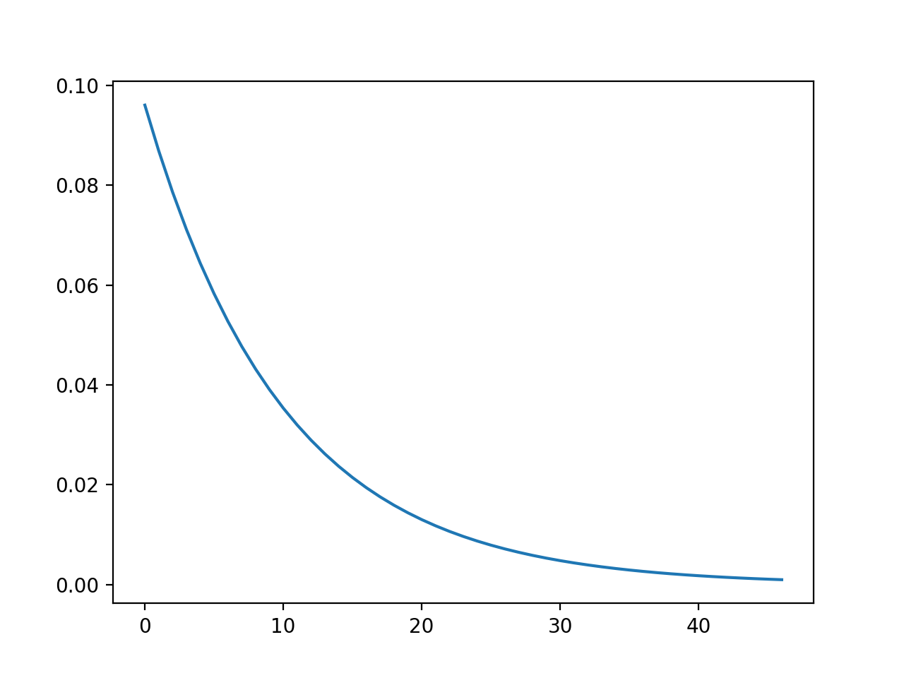
exponential(tau=0.0, adjust_padding=False, *args, **kwargs)[source]¶: Sets the weight to be a 1d temporal lowpass filter with time constant tau.

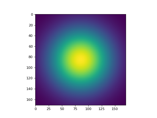
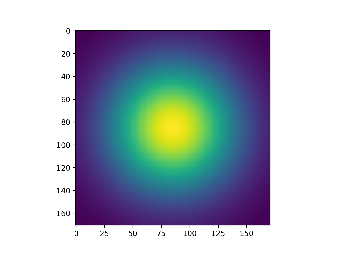
highpass_exponential(tau=0.0, adjust_padding=False, *args, **kwargs)[source]¶: Sets the weight to be a 1d temporal highpass filter with time constant tau.

gaussian(sig, adjust_padding=False, resolution=None)[source]¶: Sets the weight to be a 2d gaussian filter with width sig.

Spatial gaussian filters and temporal exponential filters can be generated with functions from the convis.numerical_filters submodule.

import convis
import numpy as np
import matplotlib.pylab as plt
plt.figure()
plt.imshow(convis.numerical_filters.gauss_filter_2d(4.0,4.0))
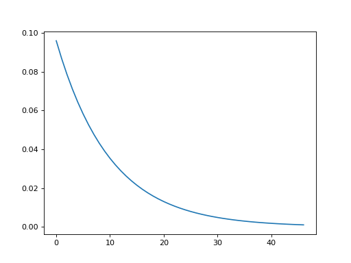
plt.figure()
plt.plot(convis.numerical_filters.exponential_filter_1d(tau=0.01))

(Source code)

(png, hires.png, pdf)

(png, hires.png, pdf)

Receptive Fields¶

While a convolution will pad the input to keep the size of the output equal to the input, a receptive field filter will produce a single time series.

class convis.filters.RF(in_channels=1, out_channels=1, kernel_size=(1, 1, 1), bias=True, rf_mode='corner', *args, **kwargs)[source]¶

A Receptive Field Layer

Does a convolution and pads the input in time with previous input, just like Conv3d, but with no spatial padding, resulting in a single output pixel.

To use it correctly, the weight should be set to the same spatial dimensions as the input. However, if the weight is larger than the input or the input is larger than the weight, the input is padded or cut. The parameter rf_mode controls the placement of the receptive field on the image.

Currently, only rf_mode=’corner’ is implemented, which keeps the top left pixel identical and only extends or cuts the right and bottom portions of the input.

Warning

The spatial extent of your weight should match your input images to get meaningful receptive fields. Otherwise the receptive field is placed at the top left corner of the input.

If the weight was not set manually, the first time the filter sees input it creates an empty weight of the matching size. However when the input size is changed, the weight does not change automatically to match new input. Use reset_weight() to reset the weight or change the size manually.

Any receptive field of size 1 by 1 pixel is considered empty and will be replaced with a uniform weight of the size of the input the next time the filter is used.

See also

torch.nn.Conv3d, Conv3d

Examples

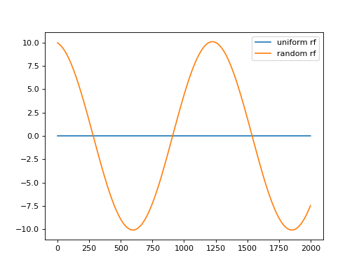
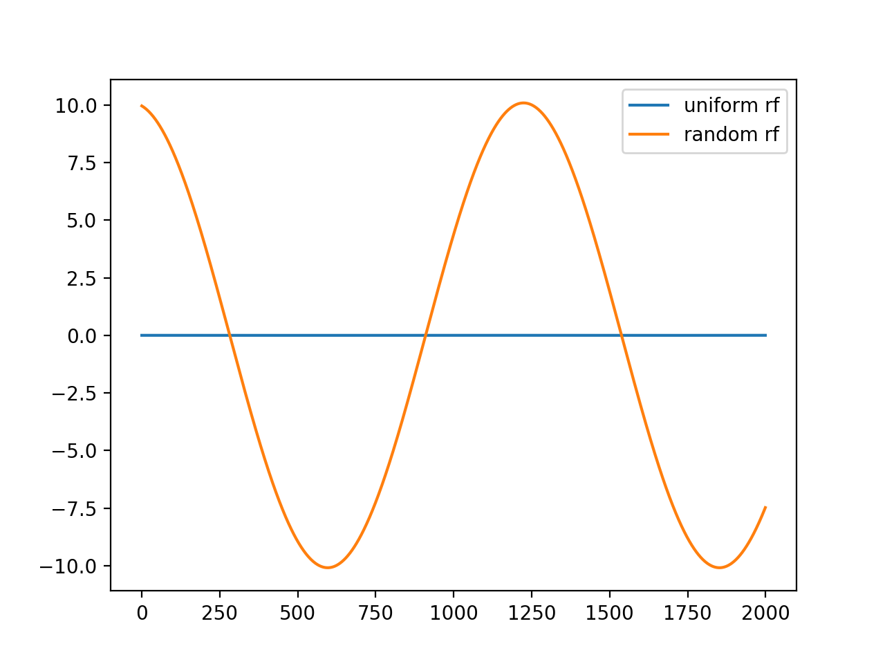
Simple usage example processing a grating stimulus from convis.samples:

>>> m = convis.filters.RF()
>>> inp = convis.samples.moving_gratings()
>>> o = m.run(inp, dt=200)
>>> o.plot()

Or as a part of a cascade model:

>>> m = convis.models.LNCascade()
>>> m.add_layer(convis.filters.Conv3d(1,5,(1,10,10)))
>>> m.add_layer(convis.filters.RF(5,1,(10,1,1)))
    # this RF will take into account 10 timesteps, it's width and height will be set by the input
>>> inp = convis.samples.moving_grating()
>>> o = m.run(inp, dt=200)

import convis
import numpy as np
import matplotlib.pylab as plt
m = convis.filters.RF()
inp = convis.samples.moving_grating()
o = m.run(inp, dt=200)
o.plot(label='uniform rf')
m.set_weight(np.random.randn(*m.weight.size()))
o = m.run(inp, dt=200)
o.plot(label='random rf')
plt.legend()

(Source code, png, hires.png, pdf)

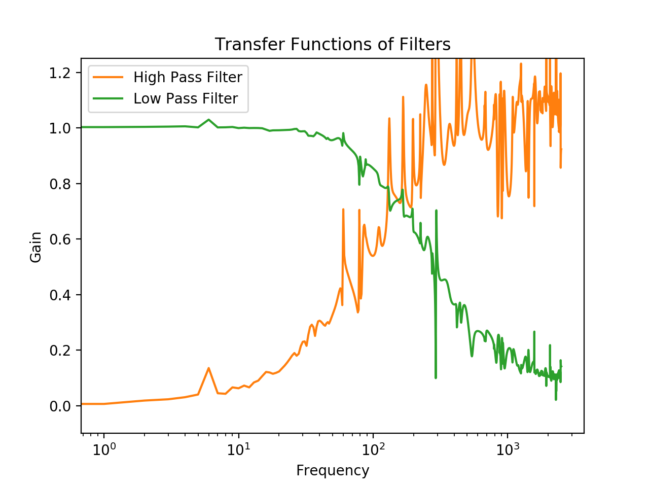
Recursive Temporal Filters¶

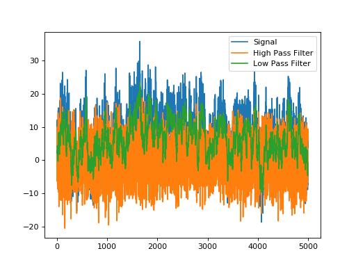
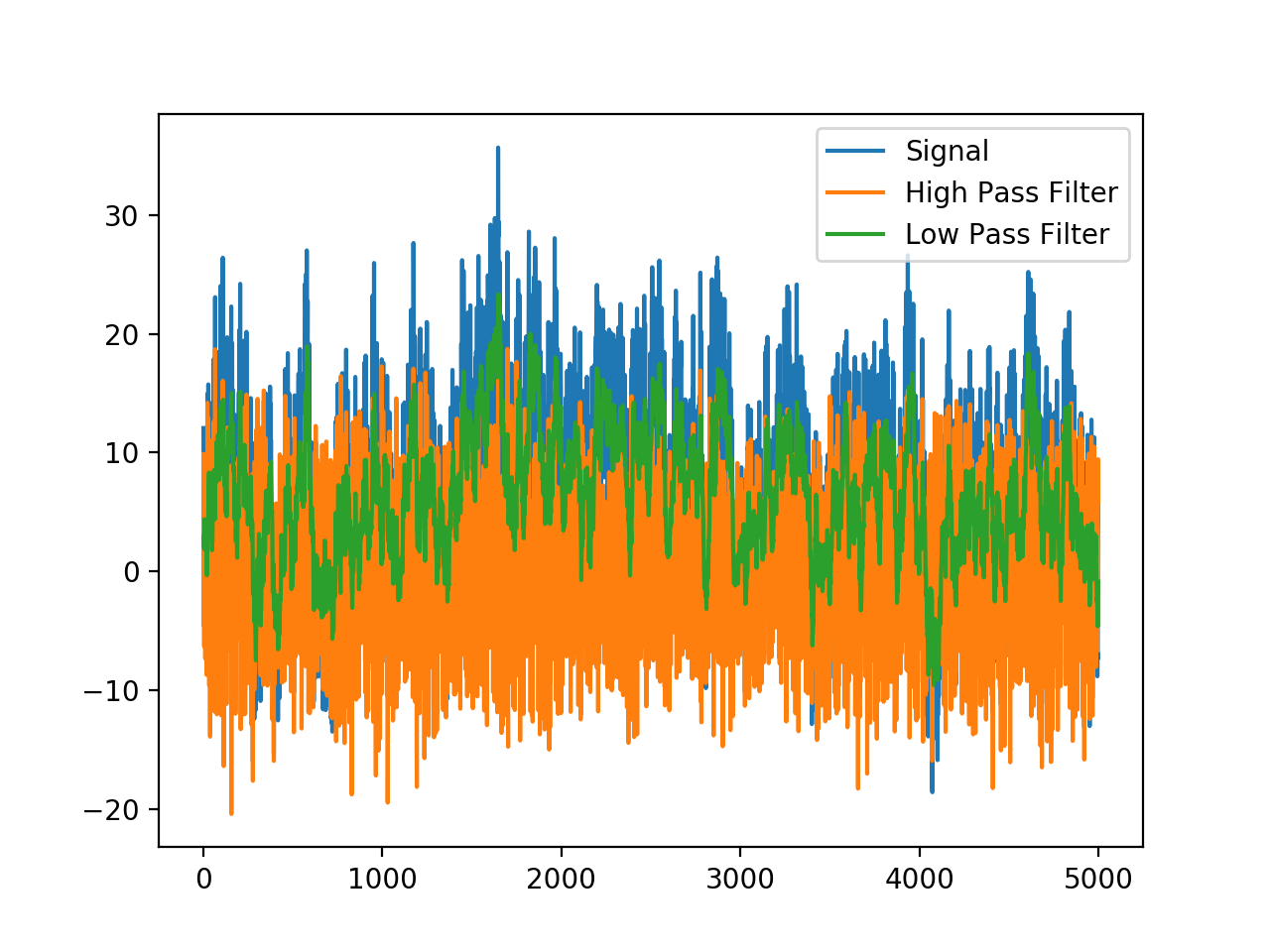
There are two filters available that perform recursive temporal filtering. The advantage over convolutional filtering is that it uses a lot less memory and is a lot faster to compute. However, the temporal filter is also more simplified and might not be able to fit a specific temporal profile well.

TemporalLowPassFilterRecursive is an exponential filter that cuts off high frequencies, while TemporalHighPassFilterRecursive is the inverse (a 1, followed by a negative exponential) and cuts off low frequencies.

import matplotlib.pyplot as plt
import numpy as np
import convis
# random amplitudes and phases for a range of frequencies
signal = np.sum([np.random.randn()*np.sin(np.linspace(0,2.0,5000)*(freq)
                 + np.random.rand()*2.0*np.pi)
                 for freq in np.logspace(-2,7,136)],0)
f1 = convis.filters.simple.TemporalLowPassFilterRecursive()
f1.tau.data[0] = 0.005
f2 = convis.filters.simple.TemporalHighPassFilterRecursive()
f2.tau.data[0] = 0.005
f2.k.data[0] = 1.0
o1 = f1(signal[None,None,:,None,None]).data.numpy().mean((0,1,3,4)).flatten()
o2 = f2(signal[None,None,:,None,None]).data.numpy().mean((0,1,3,4)).flatten()
plt.plot(signal,label='Signal')
plt.plot(o2,label='High Pass Filter')
plt.plot(o1,label='Low Pass Filter')
signal_f = np.fft.fft(signal)
o1_f = np.fft.fft(o1)
o2_f = np.fft.fft(o2)
plt.legend()
plt.figure()
plt.plot(0,0)
plt.plot(np.abs(o2_f)[:2500]/np.abs(signal_f)[:2500],label='High Pass Filter')
plt.plot(np.abs(o1_f)[:2500]/np.abs(signal_f)[:2500],label='Low Pass Filter')
plt.xlabel('Frequency')
plt.ylabel('Gain')
plt.title('Transfer Functions of Filters')
plt.gca().set_xscale('log')
plt.ylim(-0.1,1.25)
plt.legend()

(Source code)

(png, hires.png, pdf)

(png, hires.png, pdf)

Nonlinearities¶

class convis.filters.NLRectify[source]¶: Rectifies the input (ie. sets values < 0 to 0)

class convis.filters.NLRectifyScale[source]¶

Rectifies the input, but transforms the input with a scale and a bias.

Pseudocode:

out = bias + the_input * scale
out[out < 0] = 0

class convis.filters.NLSquare[source]¶: A square nonlinearity with a scalable input weight and bias.

class convis.filters.NLRectifySquare[source]¶: A square nonlinearity with a scalable input weight and bias that cuts off negative values after adding the bias.

Spike Generation¶

class convis.filters.spiking.Poisson(**kwargs)[source]¶

Poisson spiking model.

Input has to be a firing rate between 0.0 and 1.0.

New in version 0.6.4.

class convis.filters.spiking.Izhikevich(output_only_spikes=True, **kwargs)[source]¶

Izhikevich Spiking Model with uniform parameters

The Simple Model of Spiking Neurons after Eugene Izhikevich offers a wide range of neural dynamics with very few parameters.

See: https://www.izhikevich.org/publications/spikes.htm

Each pixel has two state variables: v and u. v corresponds roughly to the membrane potential of a neuron and u to a slow acting ion concentration. Both variables influence each other dynamically:

$$\dot{v} = 0.04 \cdot v^2 + 5 \cdot v + 140 - u + I$$ $$\dot{u} = a \cdot (b \cdot v - u)$$

If v crosses a threshold, it will be reset to a value c and u will be increased by another value d.

The parameters of the model are:

a: relative speed between the evolution of v and u

b: amount of influence of v over u

c: the reset value for v if it crosses threshold

d: value to add to u if v crosses threshold

Parameters:

output_only_spikes (bool)

whether only spikes should be returned (binary), or spikes, membrane potential and slow potential in one channel of the output each.

load_parameters_by_name(name=None)[source]¶

Allows to load parameters for a range of behaviors.

For a list of possible options, run the method without parameter or look at directly at the dictionary convis.filters.spiking._izhikevich_parameters.

The dictionary has values for a,b,c,d and the recommended input.

class convis.filters.spiking.RefractoryLeakyIntegrateAndFireNeuron(**kwargs)[source]¶

LIF model with refractory period.

Identical to convis.filter.retina.GanglionSpiking.

The ganglion cells recieve the gain controlled input and produce spikes.

When the cell is not refractory, $V$ moves as:

$$ \dfrac{ dV_n }{dt} = I_{Gang}(x_n,y_n,t) - g^L V_n(t) + eta_v(t)$$

Otherwise it is set to 0.

Attributes

refr_mu	(Parameter) The mean of the distribution of random refractory times (in seconds).
refr_sigma	(Parameter) The standard deviation of the refractory time that is randomly drawn around refr_mu
noise_sigma	(Parameter) Amount of noise added to the membrane potential.
g_L	(Parameter) Leak current (in Hz or dimensionless firing rate).

class convis.filters.spiking.LeakyIntegrateAndFireNeuron(**kwargs)[source]¶

LIF model.

$$ \dfrac{ dV_n }{dt} = I_{Gang}(x_n,y_n,t) - g^L V_n(t) + eta_v(t)$$

See also

RefractoryLeakyIntegrateAndFireNeuron

Attributes

noise_sigma	(Parameter) Amount of noise added to the membrane potential.
g_L	(Parameter) Leak current (in Hz or dimensionless firing rate).

class convis.filters.spiking.FitzHughNagumo(**kwargs)[source]¶

Two state neural model.

$$\dot{v} = v - \frac{1}{3} v^3 - w + I$$ $$\dot{w} = \tau \cdot (v - a - b \cdot w) $$