The API: Convis classes and modules

Table of Contents

• The API: Convis classes and modules
  • Base classes convis.base
  • Variables convis.variables
  • Utilitary methods convis.utils
  • Sample Data convis.samples
  • Methods to describe objects convis.variable_describe

Further Submodules:

• Filters convis.filters
  • Kernels convis.kernels
• Models in convis.models
  • Convis Models
  • Combinators
  • Linear-Nonlinear Models
  • Convolution Model
• Finding all Layers in one submodules convis.layers
• VirtualRetina-like Simulator
  • General Overview
  • References
  • convis.retina
  • convis.filters.retina
  • convis.retina_virtualretina
• Streams convis.streams
• Optimizers convis.optimizer
• Automatic Tests convis.tests

convis.set_steps_per_second(sps)

changes the default scaling of temporal constants.

Does not consistently work retroactively, so if you want to change it, do it before anything else.

convis.set_pixel_per_degree(ppd)

changes the default scaling of spatial constants.

Does not consistently work retroactively, so if you want to change it, do it before anything else.

Base classes convis.base

Convis base classes

Convis extends PyTorch by adding some methods to torch.nn.Module and calling it a Layer.

class convis.base.Output(outs, keys=None)

This object provides a container for output numpy arrays which are labeled with theano variables.

The outputs can be queried either by sorted order (like a simple list), by the theano variable which represents this output, the name of this variable or the full path of the variable. To make this meaningfull, provide a name to your output variables.

In the case of name collisions, the behavior of OrderedDict will use the last variable added.

The full path names of all variables are also added to this objects __dict__, allowing for tab completion.

plot(k=0, mode=None, **kwargs)

Plots the contents of the Output object.

To get a line plot:

o.plot(mode=’lines’) # default

To get a matshow plot:

o.plot(mode=’matshow’)

To get plot depending on the shape of the output:

o.plot(mode=None)

array(k=0)

Returns the contents of the Output object as a numpy array.

k: number of output (default=0)

mean(axis=None, k=0)

Computes the mean along the supplied axis.. axis = None will compute the mean over all axis.

Equivalent to:

o.array(k).mean(axis)

convis.base.prepare_input(a, dims=5, cuda=False, volatile=False, requires_grad=False, dtype='float32')

Utility function to broadcast input to 5 dimensions, make it a Tensor, wrap it in a Variable and optionally move it to the GPU.

Short hand for:

import torch
a_var = torch.autograd.Variable(torch.Tensor(a[None,None,:,:,:]), requires_grad=True).cuda()

from convis.base import prepare_input
a_var = prepare_input(a, cuda=True, requires_grad=True)

volatile is ignored for PyTorch 0.4 and above.

convis.base.shape(x)

Return the shape of a Tensor or Variable containing a Tensor.

class convis.base.Layer

Base class for modules, layers and models.

convis.Layer is a torch.nn.Module with some added functionality.

In addition to a method forward that performs the computation, a Layer object also keeps track of a state, parameter values and an optimizer.

The state is defined differently than the “state” of Module state, eg. in state_dict, includes all parameters and buffers of the model) The values of states are only important between the processing of two consecutive inputs, so they usually do not have to be saved to disk, but they have to be stored and retrieved (using get_state and set_state) when moving non-continuously over the input.

The parameters are variables of the model that have to be configured or fitted to make the model behave in the desired way. The values of these parameters define the response of the model to input and can be optimized to recreate a response observed in some data. These values can be saved to disc to preserve them.

Layers can hold an internal optimizer that makes it easy to fit the parameters of a model to data.

To create a Layer, create a subclass with an __init__ and forward method:

import convis
import torch.nn.functional as F

class Model(convis.Layer):
    def __init__(self):
        super(Model, self).__init__()
        self.conv1 = convis.filters.Conv3d(1, (20,1,1))
        self.conv2 = convis.filters.Conv3d(1, (1,10,10))
    def forward(self, x):
       x = F.relu(self.conv1(x))
       return F.relu(self.conv2(x))

Just as Module`s, `Layer`s can include other `Layer`s or `Module`s (ie. its `sublayers). Variable`s, `Parameter`s and `State`s that are attributes of a Layer or its `sublayers will be registered and can be collected according to their class.

All registered Variables (including Parameters and States), will be moved to the corresponding device when calling .cuda() or .cpu().

In contrast to many methods of torch.Tensors, Layer methods are always in-place! Using .cuda() or .float() will return a reference to the original model and not a copy.

See also

torch.nn.Module

torchs layer class

Examples

>>> import convis
>>> import torch.nn.functional as F
>>> 
>>> class Model(convis.Layer):
>>>     def __init__(self):
>>>         super(Model, self).__init__()
>>>         self.conv1 = convis.filters.Conv3d(1, (20,1,1))
>>>         self.conv2 = convis.filters.Conv3d(1, (1,10,10))
>>>     def forward(self, x):
>>>        x = F.relu(self.conv1(x))
>>>        return F.relu(self.conv2(x))

Selecting an Optimizer and using it with optimize():

>>> m = convis.models.LN()
>>> m.set_optimizer.<then press tab>
                    ASGD
                    Adadelta
                    Adagrad
                    Adam
                    ...
>>> m.set_optimizer.SGD(lr=0.01)
>>> m.optimize(input,output)

The list of parameters as first argument can be omitted and will be filled with all parameters of the model by default. Other parameters are passed through to the optimizer eg. the learning rate lr in this example.

The special attributes p,`m`,`s` and user_parameters provide tab-completion for parameters, submodules and states:

>>> retina = convis.models.retina()
>>> print retina.p
Parameters of the model (see also .user_parameters)
Choices: gang_0_spikes, gang_1_spikes, gang_0_input, gang_1_input, bipolar, opl
>>> print retina.user_parameters
Parameters of the model that can be set by the user.
Choices: gang_0_spikes, gang_1_spikes, gang_0_input, gang_1_input, bipolar, opl
>>> print retina.p
Modules of the model
Choices: _self, gang_0_spikes, gang_1_spikes, gang_0_input, gang_1_input, bipolar, opl
>>> print retina.s
Current state of the model
Choices: gang_0_spikes, gang_1_spikes, gang_0_input, gang_1_input, bipolar, opl

To find explore the parameters / modules / states, print the object to see the available choices or press tab:

>>> retina.p.<tab complete>
>>> retina.p.bi<tab complete>
>>> retina.p.bipolar.<tab complete>
>>> retina.p.bipolar.g_leak # the g_leak Parameter

The hierarchical Ox object provides a few special functions

>>> retina.p._all.bipolar_g_leak # lists everything in a flat list
>>> retina.p._search.leak.<tab complete to search>
>>> retina.p._search.leak.bipolar_g_leak # found one result

Attributes

_use_cuda	(bool)
.. py:attribute:: set_optimizer	magic object that allows tab completion to select an optimizer. (see example) The list of parameters as first argument can be omitted and will be filled with all parameters of the model by default. Other parameters are passed through to the optimizer.
.. py:attribute:: user_parameteres	A hierarchical, tab-completable list of all set() function for the user.
.. py:attribute:: m	A hierarchical, tab-completable list of all :class:`~torch.nn.Module`s/:class:`~convis.base.Layer`s of the model.
.. py:attribute:: s	A hierarchical, tab-completable list of all state variables of the model.

Methods

cuda(device=None)	move the model to the gpu
cpu()	move the model to the cpu
run(the_input, dt=None)	execute the model, using chunk sizes of dt
parse_config(conf)
optimize(inp,outp,dt=None)	use the selected optimizer to fit the model to return outp to the input inp. Accepts a chunk length dt
register_state(name, value)	registers an attribute name to be a state variable
get_state()	returns the current state of the model (recursively for all submodules)
set_state(d)	set all state parameters defined in dictionary d to the corresponding values.
push_state()	pushes the current state on a stack
pop_state()	pops the last state from the stack and sets all state variables to the corresponding values.

cuda(device=None)

Moves the model to the GPU (optionally with number device). returns the model itself.

cpu()

Moves the model to the CPU and returns the model itself.

run(the_input, dt=None, t=0, detach=True, max_t=None)

Runs the model either once, or multiple times to process chunks of size dt.

the_input can be:

• a 3d numpy.ndarray or torch.Tensor
• a convis.streams.Stream

• a Output containing at least one torch.Tensor

  • the first one will be used

Returns an Output object.

p

A hierarchical, tab-completable list of all convis.variables.Parameter of the model. If a parameters is reachable via some_model.p.layer1.module1.parameter1 it will also be available directly as some_model.layer1.module1.parameter1. However for tab-completion, the later method provides all attributes of the model, not only parameters.

See also this section in the documentation

m

A hierarchical, tab-completable list of all convis.base.Layer of the model.

s

A hierarchical, tab-completable list of all convis.variables.State of the model.

parse_config(config, prefix='', key='retina_config_key')

Loads parameter values from a configuration (RetinaConfiguration or dict).

compute_loss(inp, outp, loss_fn=<function <lambda>>, dt=None, t=0)

Computes the loss of the model output in response to inp compared with the provided outp using loss_fn.

Works like optimize, but does not use an actual optimizer.

See also

optimize

optimize(inp, outp, optimizer=None, loss_fn=<function <lambda>>, dt=None, t=0, t_skip=0)

Runs an Optimizer to fit the models parameters such that the output of the model when presented inp approximates outp.

To use this function, an torch.optim.Optimizer has to be selected:

>>> model.set_optimizer(torch.optim.SGD(model.parameters(),lr=0.01))
>>> model.optimize(x,y, dt=100)

or:

>>> model.set_optimizer.SGD(lr=0.01) # uses optimizers from torch.optim
>>> model.optimize(x,y, dt=100)

It is important to specify a chunk length dt, if the complete input does not fit into memory.

With t_skip an initial portion of the input will be evaluated by the model, without calling the optimizer.

get_parameters()

returns an OrderedDict of all parameter values of the model

The key of each entry is the respective path name (eg. ‘submodule_submodule_variablename’), the value is a numpy array.

See also

set_parameters, push_parameters, pop_parameters, save_parameters, load_parameters

set_parameters(d, warn=False)

sets parameter values from a dictionary.

All parameters of the model will be loaded according to the respective path names (eg. ‘submodule_submodule_variablename’).

Note

It is important that you load the parameters to a model with the same structure and parameters of exactly the same name! Missing parameters (either in the file or the model) will be ignored silently. To enable warnings, set Layer._debug or the argument warn to True. If you changed the model structure, you can load the parameters with np.load, convert it into a dictionary and add or rename the parameters there.

Parameters:

d (dict)

dictionary with parameter values

warn (bool)

whether to warn of mismatching parameter names

See also

get_parameters, push_parameters, pop_parameters, save_parameters, load_parameters

get_state()

collects the state and returns an OrderedDict

set_state(state_dict)

collects the state and returns an OrderedDict

requires_grad_(requires_grad)

Changes the requires_grad attribute of all contained parameters.

Setting this top False will disable the computational graph, making it impossible to use gradient descent on computations until you enable it again.

See also the documentation on how to enable/disable graphs globally, for a Layer or for a Parameter.

clear_state()

resets the state to default values

save_parameters(filename, filetype='npz')

saves the model parameters to a file

This function currently only supports the npz format. All parameters of the model will be saved as variables of the respective path names (eg. ‘submodule_submodule_variablename’).

Parameters:

filename (str)

name of the file to save to

See also

load_parameters

load_parameters(filename, filetype='npz', warn=False)

loads saved parameter values from a file.

This function currently only supports the npz format. All parameters of the model will be loaded from npz variables of the respective path names (eg. ‘submodule_submodule_variablename’).

Note

It is important that you load the parameters to a model with the same structure and parameters of exactly the same name! Missing parameters (either in the file or the model) will be ignored silently. To enable warnings, set Layer._debug or the argument warn to True. If you changed the model structure, you can load the parameters with np.load, convert it into a dictionary and add or rename the parameters there.

Parameters:

filename (str)

name of the file to load from

warn (bool)

whether to warn of mismatching parameter names

See also

save_parameters

push_parameters()

collects all parameter values and pushes their values onto a stack

pop_parameters()

retrieves the values of all parameters from a stack

push_state()

collects all State variables and pushes their values onto a stack

pop_state()

retrieves the values of all State variables from a stack

push_optimizer()

pushes the current optimizer onto a stack

pop_optimizer()

retrieves the last optimizer from a stack

get_all()

Returns the parameters, states and parameters in a dictionary.

store_all(name)

Stores parameters, states and parameter values in an internal dictionary.

retrieve_all(name)

Retrieves parameters, states and parameter values from an internal dictionary.

The entry is not deleted.

push_all()

Pushes the parameters, states and parameters onto a shared stack.

This stack does not interfere with the separate stacks of push_parameters, push_optimizer and push_state.

pop_all()

Retrieves the parameters, states and parameters from a shared stack.

This stack does not interfere with the separate stacks of pop_parameters, pop_optimizer and pop_state.

plot_impulse(shp=(500, 10, 10), dt=500)

Plots the response to a 1 bin impulse.

The state of the model is preserved (pushed to the stack and poped later).

Returns:The output of the model

Attributes

shp	(tuple(t, x, y)) the size of the stimulus. A larger stimulus will show a larger area of the impulse response
dt	(int) length of chunks when computing the response

plot_impulse_space(shp=(1, 20, 20), dt=500)

Plots the response to a 1 bin impulse.

The state of the model is preserved (pushed to the stack and poped later).

Returns:The output of the model

Attributes

shp	(tuple(t, x, y)) the size of the stimulus. A larger stimulus will show a larger area of the impulse response
dt	(int) length of chunks when computing the response

convis.base.Model

alias of Layer

class convis.base.Runner(model=None, input=None, output=None, goal=None)

Keeps track of the input and output of a model and can run or optimize it in a separate thread.

model has to be a convis.base.Layer

input should be a convis.streams.Stream that contains input data output should be a convis.streams.Stream that accepts new data when using optimize, goal has to have the same length as input and the same behaviour at the end of the stream (repeating or stop)

stop()

start()

run(length=None, **kwargs)

optimize()

Variables convis.variables

convis.variables.Variable

alias of _NewVariable

class convis.variables.Parameter(x, default=None, **kwargs)

A parameter of a model

Similar to a Variable, but by default has requires_grad set to True.

To disable the computational graph see this section in the documentation

requires_grad_(requires_grad=True)

Changes the requires_grad attribute for this parameter in place.

Setting this top False will disable the computational graph, making it impossible to use gradient descent on computations tracking back to this parameter until you enable it again.

See also the documentation on how to enable/disable graphs globally, for a Layer or for a Parameter.

convis.variables.create_Ox_from_torch_iterator_dicts(iterator, doc='')

Takes a dictionary (or iterator with key,value pairs) with dots in the keys and returns a hierarchical object.

>>> p = convis.variables.create_Ox_from_torch_iterator_dicts(retina.named_parameters())
    # the same as:
>>> p = Ox(**dict_with_dots_to_hierarchical_dict(dict(retina.named_parameters())))
>>> p.<tab complete>
>>> p.bipolar.<tab complete>
>>> p.bipolar.g_leak

convis.o.Ox objects have a few special attributes (with leading underscores) that help finding nodes in large hierarchies

>>> p._all # lists everything with underscore 
           # separating hierarchies (ie. similar
           # to `.named_parameters()`, but each works
           # as an attribute instead of a string
           # key)
>>> p._search.g_leak.<tab complete>
>>> p._search.g_leak.bipolar_g_leak

See also

convis.o.Ox

convis.variables.create_hierarchical_dict(vs, pi=0, name_sanitizer=<function save_name>)

pi: “path i” offset in the path

The path will only be used from element pi onwards

convis.variables.create_hierarchical_dict_with_nodes(vs, pi=0, name_sanitizer=<function save_name>)

name_sanitizer: eg. convis.base.save_name or str

convis.variables.create_context_O(var=None, **kwargs)

This function creates the ‘typical’ context that annotated variables can expect when defining init functions.

• var: the variable itself
• node: the node that wraps this part of the graph (providing eg. configuration options)
• get_config: a function of node that provides the configuration dictionary local to this node
• model: the model providing global options such as pixel_to_degree() and seconds_to_step()

During execution:

• input: the variable that is fed as input to the model (not the node!)

Further, if the variable has a config_key and a config_default field, two short cut functions retrieve and save the configuration value to minimize code redundancy:

• value_from_config(): retrieves the configuration value from node, falling back to config_default if no option is provided
• value_to_config(v): calls the set_config method of the node to save a configuration value (eg. when updated when optimizing)

To use these values in an init function eg:

as_parameter(T.iscalar("k"),init=lambda x: x.input.shape[0])

class convis.variables.VirtualParameter(func=None, var=None, call=None, value=None, dependencies=[], kwargs_dependencies={}, **kwargs)

VirtualParameters can generate parameter values from a dependency structure of other parameters.

Example:

a = VirtualParameter(float,value=0.1)
b = VirtualParameter(int,value=0)
v = VirtualParameter(convis2.numerical_filters.exponential_filter_5d).set_callback_arguments(tau=a,n=b)
a.set(0.01) # updating this parameter causes the function of v to be reevaluated 
plot(v.get()[0,:,0,0,0])
b.set(2) # the function is reevaluated again
plot(v.get()[0,:,0,0,0])

Utilitary methods convis.utils

convis.utils.make_tensor_5d(t)

Extends a tensor or numpy array to have exactly 5 dimensions.

In doing so, it interprets 1d tensors as being aligned in time, 2d tensors to be aligned in space, etc.

• 1d: t[None,None,:,None,None]
• 2d: t[None,None,None,:,:]
• 3d: t[None,None,:,:,:]
• 4d: t[None,:,:,:,:]
• 5d: t
• 6d and more: selects the first element of t until t has 5 dimensions

convis.utils.extend_to_match(a, b, align=None, mode='linear_ramp', end_values=0.0, dims=5)

Extends tensor a to have a shape at least as big as b.

If dims is equal to 5, make_tensor_5d() is used to add dimensions until both tensors have 5 dimensions.

By default, the first three dimensions will be padded by aligning the smaller tensor at the beginning of the larger tensor and the last two (spatial) dimensions are aligned centered in the larger tensor.

If dim is not equal to 5, all dimensions are centered.

Parameters:

a (numpy array or tensor):

the tensor being extended

b (numpy array or tensor):

the tensor with (potentially) larger dimensions

align (list or string):

if a list: determines the alignment for each dimension if a sting: gives the alignment mode for all dimensions possible values: strings starting with : ‘c’, ‘b’ and ‘e’ standing for: ‘center’, ‘begin’, ‘end’

mode (str):

see mode argument of numpy.pad() default: ‘linear_ramp’,

end_values (float):

see end_values argument of numpy.pad() default: 0.0

dims (int, specifically 5 or anything else):

if 5, tensors will be extended so that they have exactly 5 dimensions using make_tensor_5d()

Examples

To make sure both have the same shape:

>>> a = convis.utils.extend_to_match(a,b)
>>> b = convis.utils.extend_to_match(b,a)

convis.utils.subtract_tensors(a, b, align=None, dims=5)

Makes it easy to subtract two 5d tensors from each other, even if they have different shapes!

If dims is equal to 5, make_tensor_5d() is used to add dimensions until both tensors have 5 dimensions.

By default, the first three dimensions will be padded by aligning the smaller tensor at the beginning of the larger tensor and the last two (spatial) dimensions are aligned centered in the larger tensor.

If dim is not equal to 5, all dimensions are centered.

Parameters:

a (numpy array or tensor):

the first of the two tensors

b (numpy array or tensor):

the second of the two tensors

align (list or string):

if a list: determines the alignment for each dimension if a sting: gives the alignment mode for all dimensions possible values:

strings starting with : ‘c’,’b’ and ‘e’ standing for: ‘center’, ‘begin’, ‘end’

dims (int, specifically 5 or anything else):

if 5, tensors will be extended so that they have exactly 5 dimensions using make_tensor_5d()

convis.utils.plot_5d_matshow(w, border=True, dims=[(0, 1, 3), (2, 4)], border_val=0.0, **kwargs)

Plots a 5d Tensor as a concatenation of spatial maps.

The 5 dimensions have to be separated into two sets which will correspond to the two dimensions of the image.

plot_5d_matshow(w, dims=[(0,3),(2,1,4)])

Other arguments and keyword arguments are passed to matplotlib.pylab.plot()

border_val can be a float value or ‘max’, ‘min’ or ‘mean’, in which case the corresponding value will be taken from w.

Examples

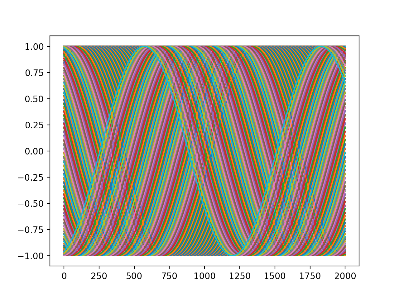
By default this will generate a very long plot where you can see almost nothing:

import convis
inp = convis.samples.moving_grating(2000,50,50)
convis.utils.plot_5d_matshow(inp[None,None])

(Source code, png, hires.png, pdf)

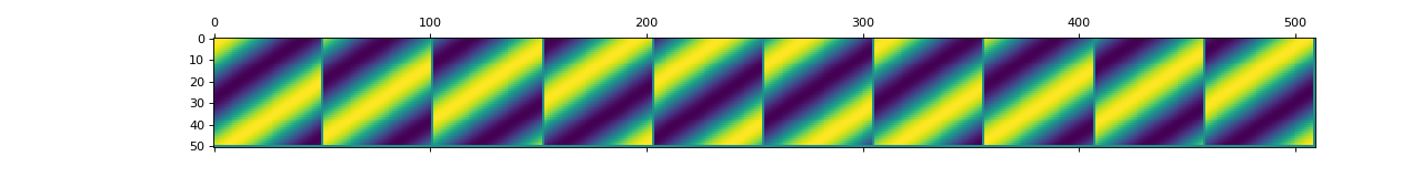
By limiting the number of frames, the plot shows the frames next to each other:

import convis
inp = convis.samples.moving_grating(2000,50,50)
convis.utils.plot_5d_matshow(inp[None,None,::200])

(Source code, png, hires.png, pdf)

convis.utils.plot_5d_time(w, lsty='-', mean=(), time=(2, ), *args, **kwargs)

Plots a line plot from a 5d tensor.

Dimensions in argument mean will be combined. If mean is True, all 4 non-time dimensions will be averaged.

Other arguments and keyword arguments are passed to matplotlib.pylab.plot()

Examples

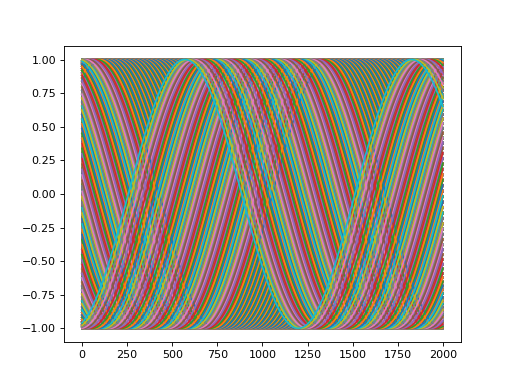
import convis
inp = convis.samples.moving_grating(2000,50,50)
convis.utils.plot_5d_time(inp[None,None])

(Source code, png, hires.png, pdf)

convis.utils.plot(x, mode=None, **kwargs)

Plots a tensor/numpy array

If the array has no spatial extend, it will draw only a single line plot. If the array has no temporal extend (and no color channels etc.), it will plot a single frame. Otherwise it will use plot_tensor.

See also

plot_tensor, plot_5d_matshow, plot_5d_time

Examples

import convis
inp = convis.samples.moving_grating(2000,50,50)
convis.utils.plot(inp[None,None])

(Source code, png, hires.png, pdf)

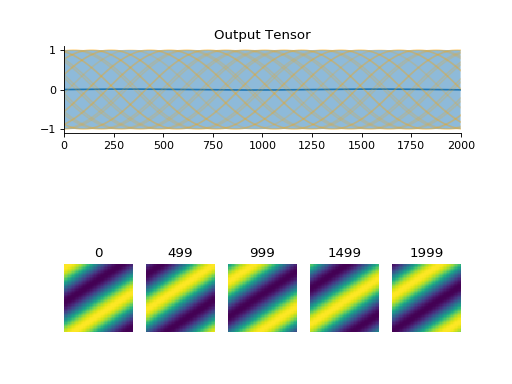
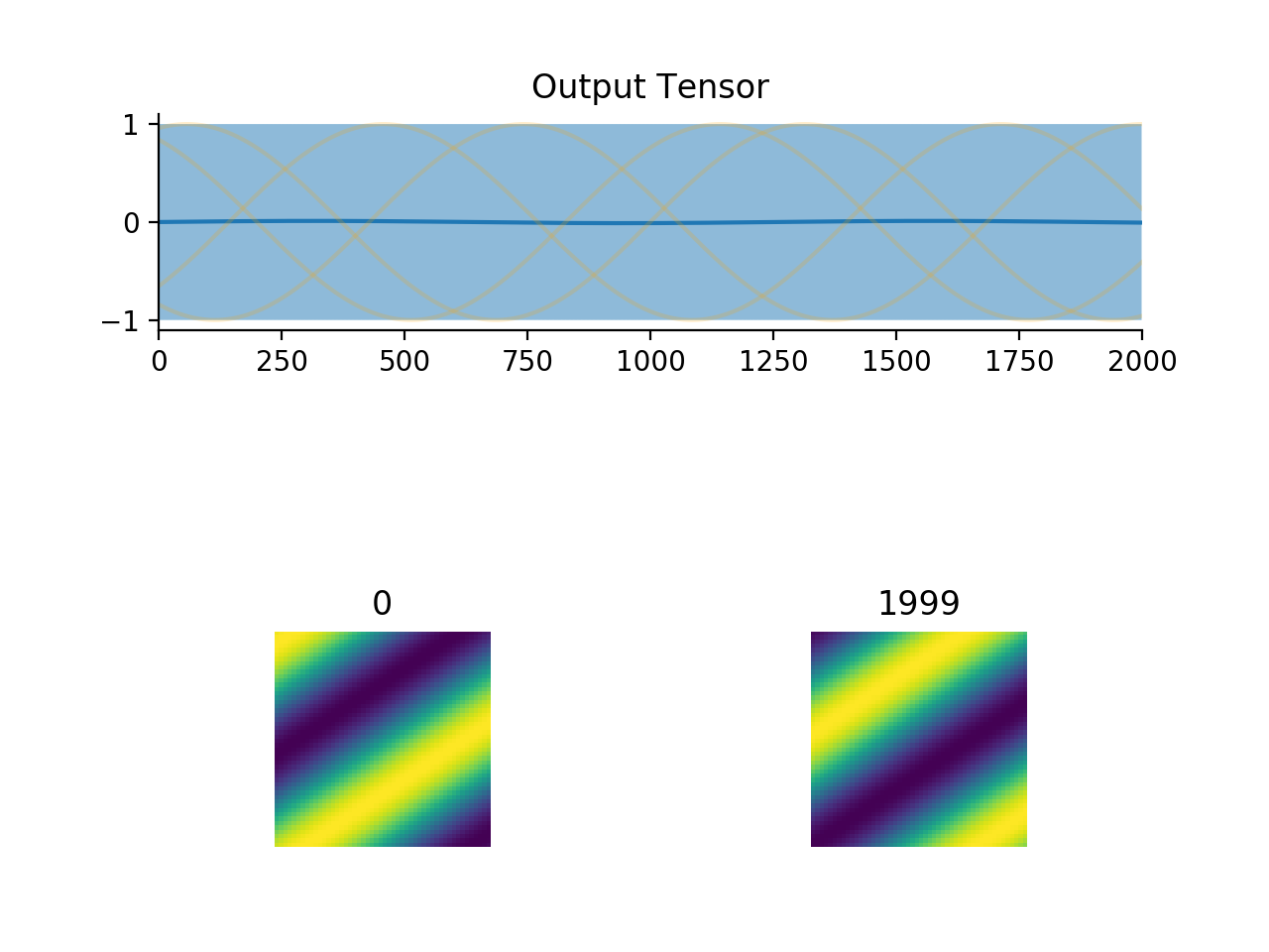
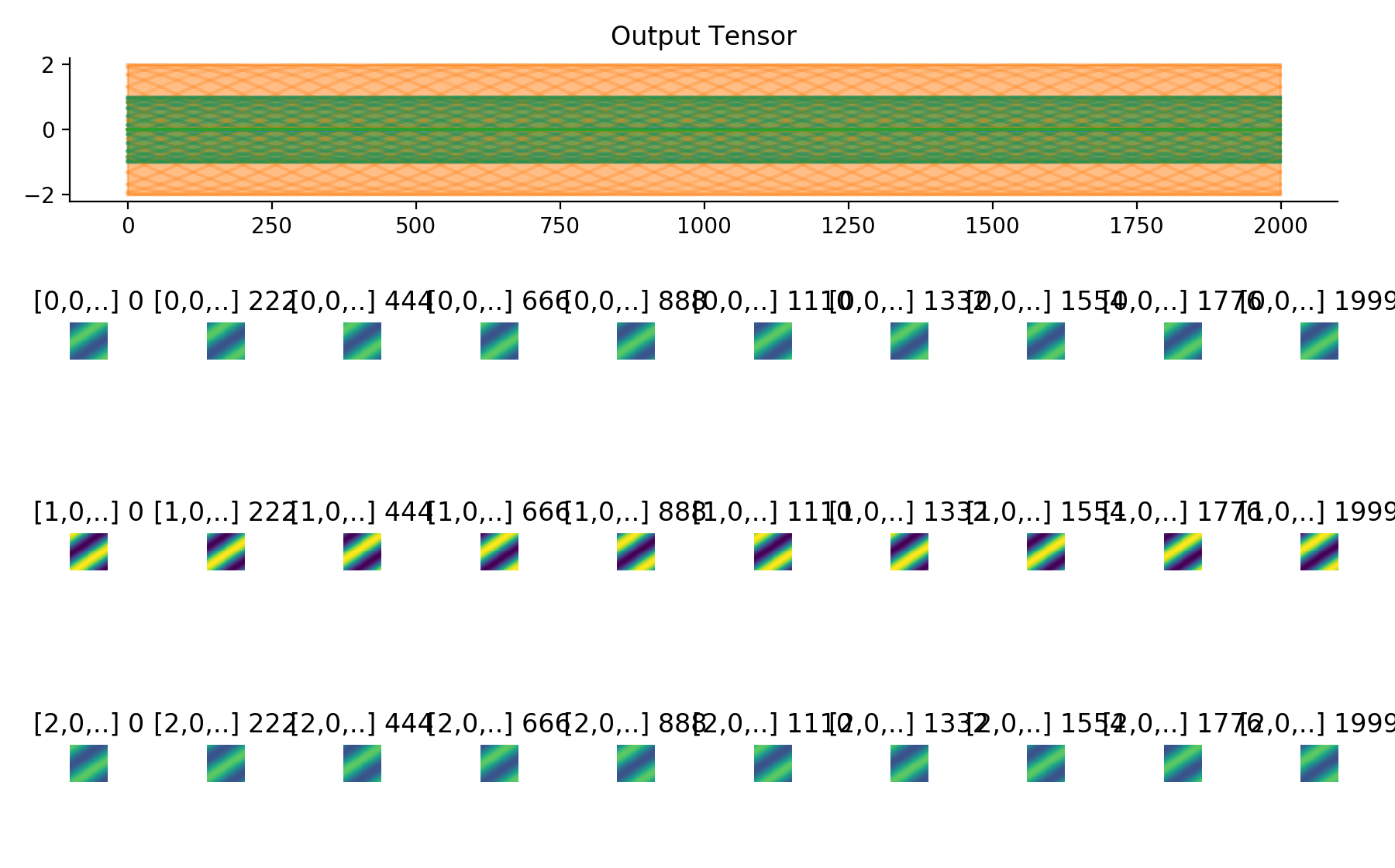
convis.utils.plot_tensor(t, n_examples=5, max_lines=16, tlim=None, xlim=None, ylim=None, resize_small_figures=True)

Plots a 5d tensor as a line plot (min,max,mean and example timeseries) and a sequence of image plots.

import convis
inp = convis.samples.moving_grating(2000,50,50)
convis.utils.plot_tensor(inp[None,None])

(Source code, png, hires.png, pdf)

Parameters:

t (numpy array or PyTorch tensor):

The tensor that should be visualized

n_examples (int):

how many frames (distributed equally over the length of the tensor) should be

max_lines (int):

the maximum number of line plots of exemplary timeseries that should be added to the temporal plot. The lines will be distributed roughly equally. If the tensor is not square in time (x!=y) or either dimension is too small, it is possible that there will be less than max_lines lines.

tlim (tuple or int):

time range included in the plot

xlim (tuple or int):

x range included in the example frames

ylim (tuple or int):

y range included in the example frames

resize_small_figures (bool):

if True, figures that do not fit the example plots will be resized

Examples

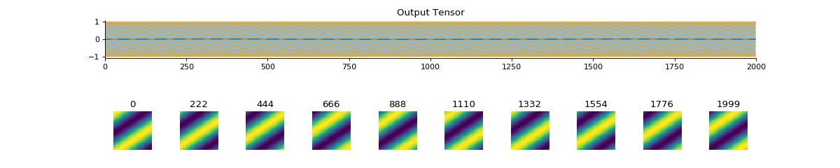
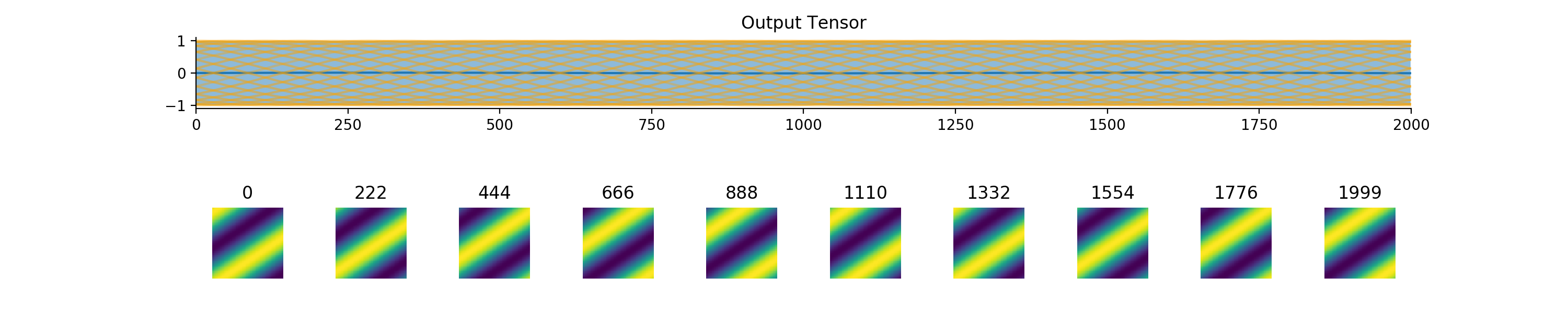
import convis
inp = convis.samples.moving_grating(2000,50,50)
convis.utils.plot_tensor(inp[None,None],n_examples=10,max_lines=42)

(Source code, png, hires.png, pdf)

import convis
inp = convis.samples.moving_grating(2000,50,50)
convis.utils.plot_tensor(inp[None,None],n_examples=2,max_lines=2)

(Source code, png, hires.png, pdf)

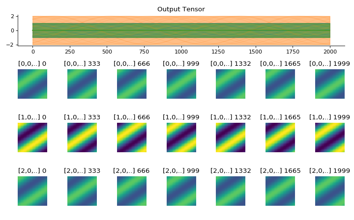
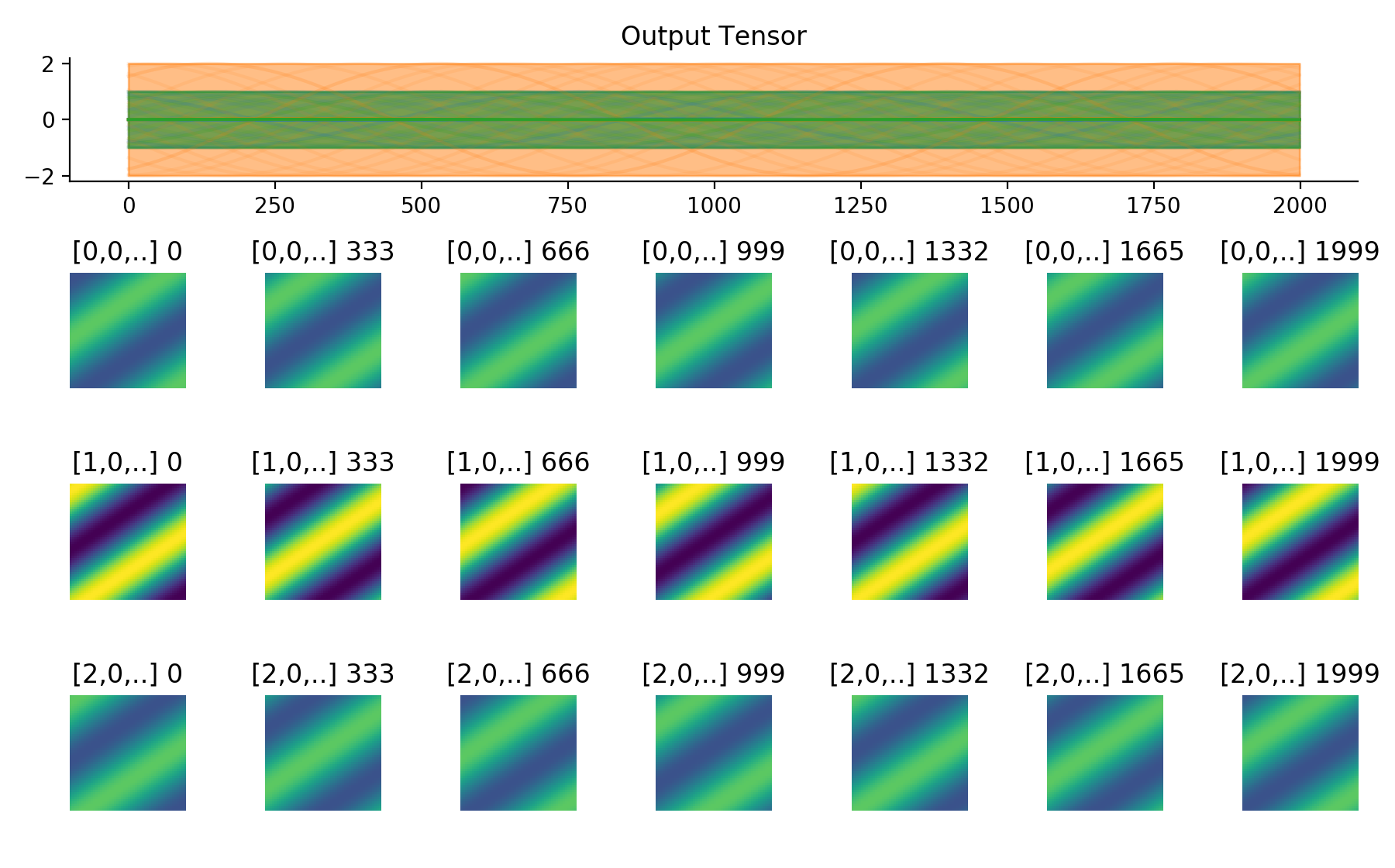
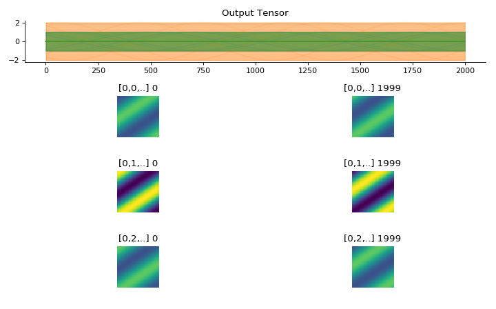
convis.utils.plot_tensor_with_channels(t, n_examples=7, max_lines=9)

Plots a 5d tensor as a line plot (min,max,mean and example timeseries) and a sequence of image plots and respects channels and batches.

(might replace plot_tensor if it is more reliable and looks nicer)

import convis
inp = convis.samples.moving_grating(2000,50,50)
inp = np.concatenate([-1.0*inp[None,None],2.0*inp[None,None],inp[None,None]],axis=0)
convis.utils.plot_tensor_with_channels(inp)

(Source code, png, hires.png, pdf)

Parameters:

t (numpy array or PyTorch tensor):

The tensor that should be visualized

n_examples (int):

how many frames (distributed equally over the length of the tensor) should be

max_lines (int):

the maximum number of line plots of exemplary timeseries that should be added to the temporal plot. The lines will be distributed roughly equally. If the tensor is not square in time (x!=y) or either dimension is too small, it is possible that there will be less than max_lines lines.

Examples

import convis
inp = convis.samples.moving_grating(2000,50,50)
inp = np.concatenate([-1.0*inp[None,None],2.0*inp[None,None],inp[None,None]],axis=0)
convis.utils.plot_tensor_with_channels(inp,n_examples=10,max_lines=42)

(Source code, png, hires.png, pdf)

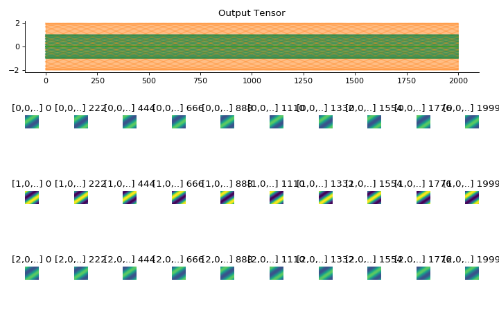
import convis
inp = convis.samples.moving_grating(2000,50,50)
inp = np.concatenate([-1.0*inp[None,None],2.0*inp[None,None],inp[None,None]],axis=1)
convis.utils.plot_tensor_with_channels(inp[None,None],n_examples=2,max_lines=2)

(Source code, png, hires.png, pdf)

Sample Data convis.samples

See also this notebook for sample stimuli.

This module provides sample kernels and inputs.

convis.samples.moving_grating(t=2000, x=20, y=20, vt=0.005, vx=3.0, vy=2.0, p=0.01, frames_per_second=None, pixel_per_degree=None)

Creates a moving grating stimulus. The actual speed and direction of the gratings is a combination of temporal, x and y speed.

Parameters:

t: int

temporal length of the stimulus

x: int

width of the stimulus

y: int

height of the stimulus

vt: float

speed of gratings

vx: float

x speed of gratings

vy: float

y speed of gratings

convis.samples.moving_bar(t=2000, x=20, y=20, bar_pos=-1.0, bar_direction=0.0, bar_width=1.0, bar_v=0.01, frames_per_second=None, pixel_per_degree=None, sharp=False, temporal_smoothing=1.0)

Creates a moving bar stimulus. By default, this bar is smoothed in time, ie. its fuzzyness is determined by its speed and temporal_smoothing.

Parameters:

t: int

temporal length of the stimulus

x: int

width of the stimulus

y: int

height of the stimulus

bar_pos: float

position of the bar from -1.0 to 1.0

bar_direction: float

direction of the bar in rad

bar_width: float

width of the bar in pixel

bar_v: float

speed of the bar

sharp: bool

whether the output is binary or smoothed

temporal_smoothing: float

if greater than 0.0 and sharp=False, smooths the stimulus in time with a gaussian kernel with width temporal_smoothing.

convis.samples.random_checker_stimulus(t=2000, x=20, y=20, checker_size=5, seed=123, frames_per_second=None, pixel_per_degree=None)

Creates a random checker flicker of uniformly distributed values in a grid of checker_size`x`checker_size pixels.

class convis.samples.StimulusSize(t=2000, x=20, y=20, pixel_per_degree=10, frames_per_second=1000.0, cuda=False, prepare=False)

This class holds information about sample stimulus size.

class convis.samples.SampleGenerator(kernel='random', kernel_size=(10, 5, 5), dt=100, p=0.1)

A Linear-Nonlinear model with a random kernel/weight that generates random input/output combinations for testing purposes.

Parameters:

kernel : str or numpy array

Possible values for kernel:

‘random’ or ‘randn’: normal distributed kernel values

‘rand’: random kernel values bounded between 0 and 1

‘sparse’: a kernel with a ratio of (approx).

p 1s and 1-p 0s, randomly assigned.

or a 5d or 3d numpy array

kernel_size : tuple(int,int,int)

specifies the dimensions of the generated input

dt : int

length of chunks when evaluating the model

p : float

the ratio of 1s for sparse input

See also

convis.samples.generate_sample_data

Examples

>>> g = convis.samples.SampleGenerator('sparse',kernel_size=(20,5,5),p=0.05)
>>> x,y = g.generate()
>>> m = convis.models.LN((50,10,10))
>>> m.set_optimizer.Adam()
>>> m.optimize(x,y)

Attributes

conv	(convis.filters.Conv3d) the convolution operation (including the weight)

Methods

generate(input,size,p)

generates random input and corresponding output

generate(input='random', size=(2000, 20, 20), p=0.1)

Parameters:

input : str or numpy array

Possible values for input:

• ‘random’ or ‘randn’: normal distributed input
• ‘rand’: random input values bounded between 0 and 1

• ‘sparse’: input with a ratio of (approx).

  p 1s and 1-p 0s, randomly assigned.

• or a 3d or 5d numpy array.

If input is anything else, generate tries to use it as input to the model.

size : tuple(int,int,int)

specifies the dimensions of the generated input

p : float

the ratio of 1s for sparse input

Returns:

x : PyTorch Tensor

the randomly created input input

y : PyTorch Variable

the corresponding output

convis.samples.generate_sample_data(input='random', size=(2000, 20, 20))

Generates random input and sample output using a SampleGenerator with a random kernel.

Parameters:

input : str or numpy array

Possible values for input:

• ‘random’ or ‘randn’: normal distributed input
• ‘rand’: random input values bounded between 0 and 1

• ‘sparse’: input with a ratio of (approx).

  p 1s and 1-p 0s, randomly assigned.

• or a 3d or 5d numpy array.

size : tuple(int,int,int)

specifies the dimensions of the generated input

Returns:

x : PyTorch Tensor

the randomly created input input

y : PyTorch Variable

the corresponding output

The kernel will be different each time

convis is (re)loaded, but constant in one

session. The “secret” SampleGenerator is

available as convis.samples._g.

See also

SampleGenerator

Examples

>>> m = convis.models.LN((50,10,10))
>>> m.set_optimizer.Adam()
>>> x,y = convis.samples.generate_sample_data()
>>> m.optimize(x,y)

Methods to describe objects convis.variable_describe

• Describing Variables: describe()
• Aniamting Tensors: animate(), animate_to_video()
• Plotting Tensors: plot_3d_tensor_as_3d_plot()

convis.variable_describe.describe(v, **kwargs)

All-purpose function to describe many convis objects

The output adapts itself to being displayed in a notebook or text console.

convis.variable_describe.animate(ar, skip=10, interval=100)

animates a 3d or 5d array in a jupyter notebook

Returns a matplotlib animation object.

Parameters:

ar (np.array):

3d or 5d array to animate

skip (int):

the animation skips this many timesteps between two frames. When generating an html plot or video for long sequences, this should be set to a higher value to keep the video short

interval (int):

number of milliseconds between two animation frames

See also

convis.variable_describe.animate_double_plot, convis.variable_describe.animate_to_video, convis.variable_describe.animate_to_html

Examples

To use in a jupyter notebook, use a suitable matplotlib backend:

>>> %matplotlib notebook
>>> import convis
>>> inp = convis.samples.moving_grating(5000)
>>> convis.animate(inp)
<matplotlib.animation.FuncAnimation at 0x7f99d1d88750>

To get a html embedded video, use convis.variable_describe.animate_to_video

>>> %matplotlib notebook
>>> import convis
>>> inp = convis.samples.moving_grating(5000)
>>> convis.variable_describe.animate_to_video(inp)
<HTML video embedded in the notebook>

convis.variable_describe.animate_double_plot(ar, skip=10, interval=200, window_length=200)

animates two plots to show a 3d or 5d array: a spatial and a temporal scrolling line plot

5d arrays will be converted into 3d arrays by concatenating the batch and channel dimensions in the x and y spatial dimensions.

Parameters:

ar (np.array):

3d or 5d array to animate

skip (int):

the animation skips this many timesteps between two frames. When generating an html plot or video for long sequences, this should be set to a higher value to keep the video short

interval (int):

number of milliseconds between two animation frames

window_length (int):

length of the window displayed in the scrolling line plot

See also

convis.variable_describe.animate

convis.variable_describe.animate_to_video(ar, skip=10, interval=100, scrolling_plot=False, window_length=200)

animates a 3d or 5d array in a jupyter notebook

Returns a Jupyter HTML object containing an embedded video that can be downloaded.

Parameters:

ar (np.array):

3d or 5d array to animate

skip (int):

the animation skips this many timesteps between two frames. When generating an html plot or video for long sequences, this should be set to a higher value to keep the video short

interval (int):

number of milliseconds between two animation frames

scrolling_plot (bool):

whether to plot the spatial and temporal plots or only the spatial animation

window_length (int):

if scrolling_plot is True, specifies the length of the time window displayed

See also

convis.variable_describe.animate

Examples

>>> %matplotlib notebook
>>> import convis
>>> inp = convis.samples.moving_grating(5000)
>>> convis.variable_describe.animate_to_video(inp)
<HTML video embedded in the notebook>

convis.variable_describe.animate_to_html(ar, skip=10, interval=100, scrolling_plot=False, window_length=200)

animates a 3d or 5d array in a jupyter notebook

Returns a Jupyter HTML object containing an embedded javascript animated plot.

Parameters:

ar (np.array):

3d or 5d array to animate

skip (int):

the animation skips this many timesteps between two frames. When generating an html plot or video for long sequences, this should be set to a higher value to keep the video short

interval (int):

number of milliseconds between two animation frames

scrolling_plot (bool):

whether to plot the spatial and temporal plots or only the spatial animation

window_length (int):

if scrolling_plot is True, specifies the length of the time window displayed

See also

convis.variable_describe.animate

Examples

>>> %matplotlib notebook
>>> import convis
>>> inp = convis.samples.moving_grating(5000)
>>> convis.variable_describe.animate_to_html(inp)
<HTML javascript plot embedded in the notebook>

class convis.variable_describe.OrthographicWrapper

This context manager overwrites the persp_transformation function of proj3d to perform orthographic projections. Plots that are show()n or save()d in this context will use the projection.

After the context closes, the old projection is restored.

Examples

>>> with convis.variable_describe.OrthographicWrapper():
 ..     plot_3d_tensor_as_3d_plot(ar) # orthographic projection
>>> plot_3d_tensor_as_3d_plot(ar) # returns to default projection

>>> orth = convis.variable_describe.OrthographicWrapper():
>>> with orth:
 ..     plot_3d_tensor_as_3d_plot(ar) 
>>> plot_3d_tensor_as_3d_plot(ar)

convis.variable_describe.plot_3d_tensor_as_3d_plot(ar, ax=None, scale_ar=None, num_levels=20, contour_cmap='coolwarm_r', contourf_cmap='gray', view=(25, 65))

Until I come up with a 3d contour plot that shows the contours of a volume, this function visualizes a sequence of images as contour plots stacked on top of each other. The sides of the plot show a projection onto the xz and yz planes (at index 0).

ar:

the array to visualize

ax: (if available)

the matplotlib axis (in projection=‘3d’ mode) from eg. calling subplot if none is provided, the current axis will be converted to 3d projection

scale_ar:

the array that is used for scaling (usefull if comparing arrays or visualizing only a small section)

num_levels:

number of levels of contours

contour_cmap=’coolwarm_r’:

color map used for line contours

contourf_cmap=’gray’:

color map used for surface contour

view:

tuple of two floats that give the azimuth and angle of the projection

returns:

axis that was used for plotting