Examples

There are two quickstart examples that show how to use Convis for the two main use cases it was designed for:

• “I want to convert luminance into spikes”
• “I’m an experimentalist and I want to fit models to my data”
• “I need spiking activity that looks like it’s coming from the retina”

Quickstart: Generating Spikes

import convis
import numpy as np
some_input = convis.samples.moving_grating()
spk = convis.filters.spiking.LeakyIntegrateAndFireNeuron()
spk.p.g_L = 1.0
o = spk.run(20.0*some_input,dt=100)
plt.figure()
o.plot(mode='lines')

(Source code, png, hires.png, pdf)

Quickstart: Fitting models to data

Note

You can find this example as a notebook in the example folder.

First, you need to get your data in a certain format:

• videos or stimuli can be time by x by y numpy arrays, or 1 by channel by time by x by y.
• all sequences have to have the same sampling frequency (bin-length)
• if you want to fit a spike train and you only have the spike times, you need to convert them into a time sequence

For this example we get a sample pair of input and output (which is generated by a randomized LN model):

import convis
inp, out = convis.samples.generate_sample_data(input='random',size=(2000,20,20))
print(inp.shape)

Then, you need to choose a model, eg. an LN model as well. For the LN cascade models in Convis, you can set a parameter population depending on whether you have a single or multiple responses that you want to fit. If population is True, the model will output an image at the last stage, if population is False, it will only return a time series. Our sample output is an image with the same size as the input, so population should be True (which is also the default). We also choose the size of the kernel that is used for the convolution.

m = convis.models.LN(kernel_dim=(12,10,10),population=False)

This example is not a very hard task, since the model that generated the data is very similar to the model we are fitting it with.

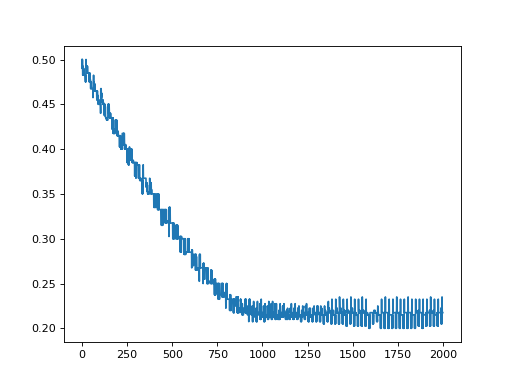
We can have a look at how well our model is doing right now by looking at the loss:

print(m.compute_loss(inp,out,dt=500))

The default loss function is the sum of squared errors, but any loss function can be used by supplying it as an argument (see optimize()). Since we didn’t fit the parameters so far, the loss will be pretty bad (around $10^7$). compute_loss returns the loss for each chunk that is computed separately. You can add them up or take the mean using np.sum or np.mean.

Next, we will choose an optimizer. Which optimizer works best for you will depend on the complexity of you model and the data you supply. We recommend trying out different ones. In this example, we will choose the Adam optimizer. A list of all optimizers can be tab-completed in IPython and jupyter notebooks when typing m.set_optimizer. and then pressing TAB.

m.set_optimizer.Adam()

Then, we can optimize the model using our complete input, but separated into smaller chunks of length dt (to make sure everything fits into memory). Most optimization algorithms need to be run more than once since they only take small steps in the direction of the gradient.

for i in range(10):
    m.optimize(inp,out,dt=500)

We can examine the loss again after a few steps of fitting and also visualize the filters. convis.plot_5d_matshow() can plot a 5 dimensional filter as a sequence of images. Since we created a filter spanning 10 frames, we see 12 little matrices, separated by a 1px border.

print(m.compute_loss(inp,out,dt=500))
convis.plot_5d_matshow(m.p.conv.weight)
title('Filter after fitting')

The loss hopefully is now lower, but it will not be decreased by very much.

To compare this result visually to the true kernel of the sample data generator we can cheat a little and look at its parameter:

convis.plot_5d_matshow(convis.samples._g.conv.weight)

Let’s use a different algorithm to optimize our parameters. LBFGS is a pseudo-Newton method and will evaluate the model multiple times per step. We do not necessarily have to run it multiple times over the data ourselves and in some cases running this optimizer too often can deteriorate our solution again, as the small gradients close to the real solution lead to numerical instabilities.

m.set_optimizer.LBFGS()
m.optimize(inp,out,dt=500)

Did we improve?

print(m.compute_loss(inp,out,dt=500))
convis.plot_5d_matshow(m.p.conv.weight)
title('Filter after fitting')

We can see clearly now that the size of our fitted kernel does not match the sample generator, which makes sense, since we normally don’t have access to a ground-truth at all. But our model just set the border pixels and the first two frames to 0.

You can use impulse responses to quickly compare Models independent of their kernel sizes. (however, for more complex models this will not capture the complete model response):

m.plot_impulse_space()
convis.samples._g.plot_impulse_space()

Finally, you can save the parameters into a compressed numpy file.

m.save_parameters('fitted_model.npz')

Quickstart: Running Convis as a simulator

Convis comes with a retina simulator. So to generate retina ganglion cell like spikes, you just have to instantiate that model and feed it with some input:

>>> import convis
>>> retina = convis.retina.Retina()

If you have a VirtualRetina xml configuration file, you can set the parameters accordingly:

>>> retina.parse_config('path/to/config_file.xml')

By default, the model has an On and an Off layer of cells with otherwise symmetric properties.

To load a sequence of images or a video, you can use a stream class:

>>> inp = convis.streams.ImageSequence('input_*.jpg')
# or
>>> inp = convis.streams.VideoReader('a_video.mp4')
# or
>>> inp = np.random.randn(2000,50,50)

Once you have your input, you can run the model. Since the input can be very long and you will most probably have a a finite amount of memory (unless you run Convis on a true Turing machine), you can specify a chunk length dt to split up the input into smaller batches.

>>> o = retina.run(inp, dt=500)

The output is collected in an Output object, which gives you access to both neural populations (On and Off cells) either by numerical index or named attributes:

>>> o[0] is o.ganglion_spikes_ON
True
>>> o[1] is o.ganglion_spikes_OFF
True

>>> convis.plot_5d_time(o[0],mean=(3,4))
>>> convis.plot_5d_time(o[1],mean=(3,4))
>>> plt.title('Firing Rates')

Running a Model

An LN Filter:

import convis
the_input = convis.samples.moving_bars(2000)

m = convis.models.LN()
o = m.run(the_input)

The premade retina model can be instanciated and executed like this:

import convis
m = convis.retina.Retina()
m.run(the_input)

If the input is very long, it can be broken into chunks:

m.run(the_input,dt=1000) # takes 1000 timesteps at a time

A runner runs in its own thread and consumes an input stream:

import convis
model = convis.retina.Retina()
input_stream = convis.streams.RandomStream(size=(50,50))
output_stream = convis.streams.InrImageStreamWriter('output.inr')
runner = convis.Runner(model,input_stream,output_stream)
runner.start()

The input stream can be infinite in length (as eg. the RandomStream), see convis.streams.

More information specific to the retina model can be found here.