VirtualRetina-like Simulator
The Retina model combines filters from
convis.filters.retina into a complete model, similar
to VirtualRetina [Wohrer2009].
To load the same xml configuration as VirtualRetina, the
module convis.retina_virtualretina provides a
RetinaConfiguration object
and a default configuration.
General Overview
The layers that create the model are:
The formulas on which the classes are based are:
OPL transforms the input with set of
linear filters to a center signal \(C\) and a surround signal \(S\)
which is subtracted to get the output current \(I_{OLP}\):
$$C(x,y,t) = G * T(wu,Tu) * E(n,t) * L (x,y,t)$$
$$S(x,y,t) = G * E * C(x,y,t)$$
$$I_{OLP}(x,y,t) = \lambda_{OPL}(C(x,y,t) - w_{OPL} S(x,y,t)_)$$
\(L\) is the luminance input,
\(G\) are spatial (different) filters,
\(T\) and \(E\) are temporal filters,
\(\lambda_{OPL}\) and \(w_{OPL}\) are scalar weights.
Subscripts of the filters are omitted (\(G\) instead of \(G_C\)),
but they should be thought of as each being a specific, unique filter.
Here \(*\) is a convolution operator.
Bipolar implements contrast gain control with a differential equation:
$$\frac{dV_{Bip}}{dt} (x,y,t) = I_{OLP}(x,y,t) - g_{A}(x,y,t)dV_{Bip}(x,y,t)$$
- with \(g_{A}(x,y,t) = G * E * Q(V{Bip})(x,y,t)\)
- and \(Q(V{Bip}) = g_{A}^{0} + \lambda_{A}V^2_{Bip}\)
- \(G\) and \(E\) are again filters
GanglionInput applies a static nonlinearity and another spatial linear filter:
$$I_{Gang}(x,y,t) = G * N(T * V_{Bip})$$
- with \(N(V) = \frac{i^0_G}{1-\lambda(V-v^0_G)/i^0_G}\) if \(V < v^0_G\)
- and \(N(V) = i^0_G + \lambda(V-v^0_G)\) if \(V > v^0_G\)
And finally a spiking mechanism GanglionSpiking is implemented by another differential equation:
$$ \dfrac{ dV(x,y) }{dt} = I_{Gang}(x,y,t) - g^L V(x,y,t) + \eta_v(t)$$
- \(V\) values above 1 set a refractory variable to a randomly drawn value
- while the refractory value is larger than 0, \(V\) of that pixel is set to 0 and the refractory variable is decremented
References
| [Wohrer2009] | Wohrer, A., & Kornprobst, P. (2009). Virtual Retina: a biological retina model and simulator, with contrast gain control. Journal of Computational Neuroscience, 26(2), 219-49. http://doi.org/10.1007/s10827-008-0108-4 |
convis.retina
This module provides the retina model.
-
class
convis.retina.Retina(opl=True, bipolar=True, gang=True, spikes=True)[source]¶ A retinal ganglion cell model comparable to VirtualRetina [Wohrer200923].
[Wohrer200923] Wohrer, A., & Kornprobst, P. (2009). Virtual Retina: a biological retina model and simulator, with contrast gain control. Journal of Computational Neuroscience, 26(2), 219-49. http://doi.org/10.1007/s10827-008-0108-4 See also
convis.base.Layer- The Layer base class, providing chunking and optimization
convis.filters.retina.OPL- The outer plexiform layer performs luminance to contrast conversion
convis.filters.retina.Bipolar- provides contrast gain control
convis.filters.retina.GanglionInput- provides a static non-linearity and a last spatial integration
convis.filters.retina.GanglionSpiking- creates spikes from an input current
Examples
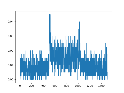
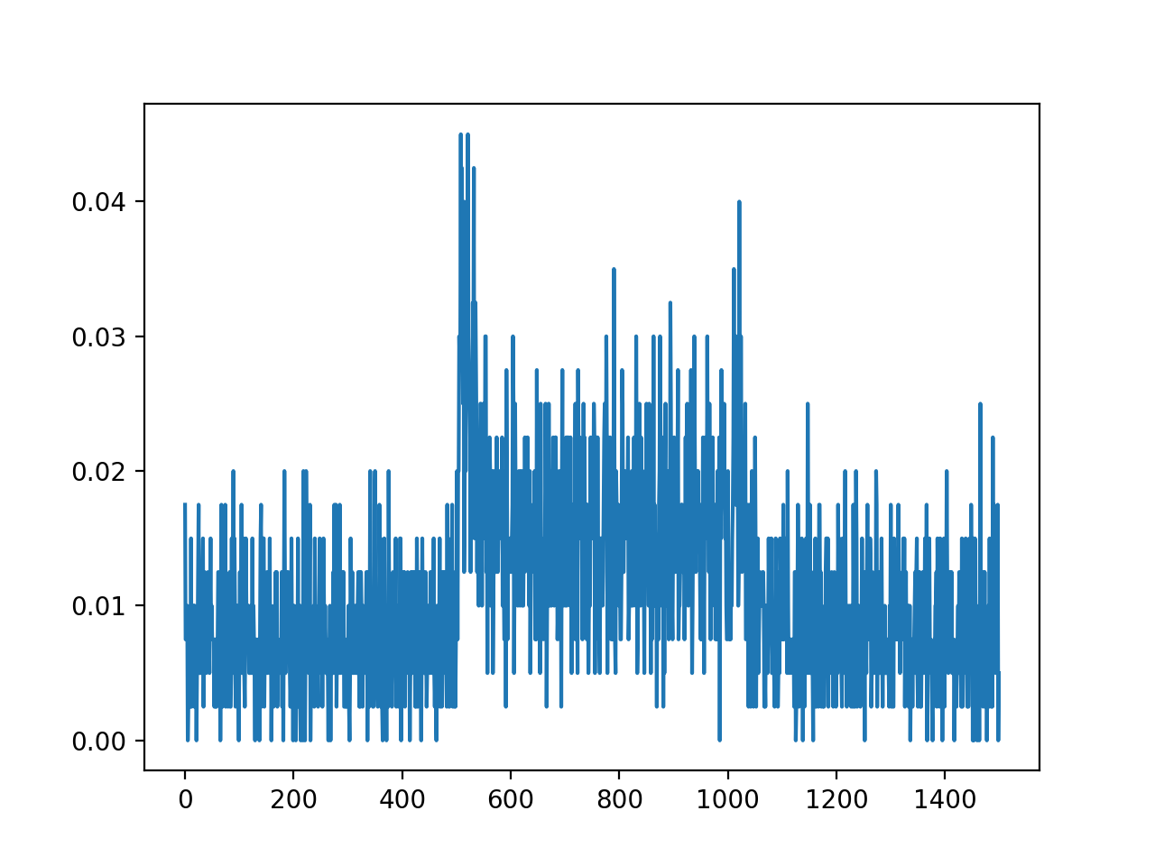
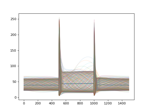
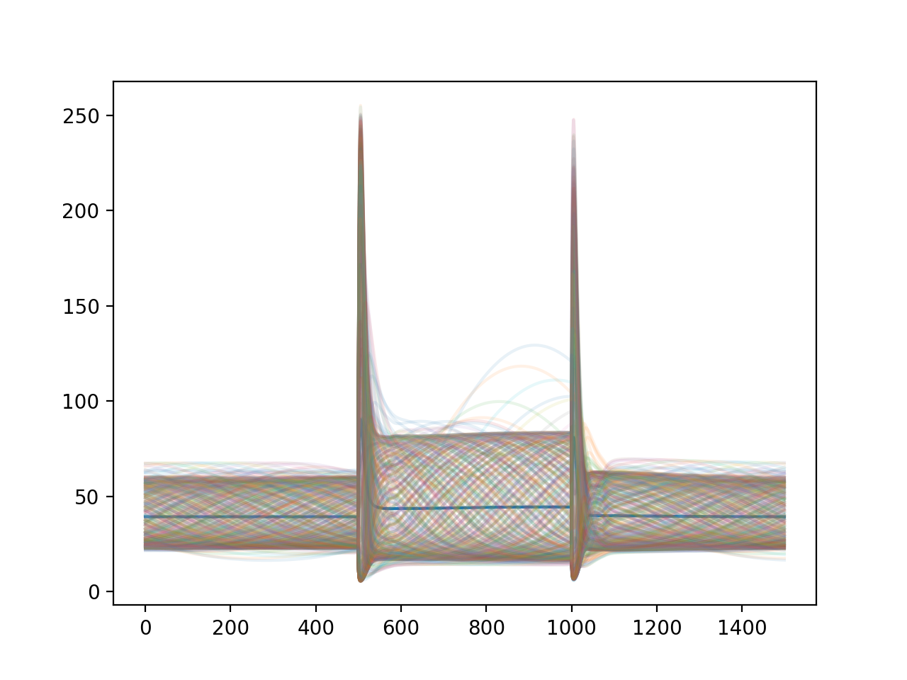
import convis
import numpy as np
from matplotlib import pylab as plt
retina = convis.retina.Retina()
inp = convis.samples.moving_grating(2000)
inp = np.concatenate([inp[:1000],2.0*inp[1000:1500],inp[1500:2000]],axis=0)
o_init = retina.run(inp[:500],dt=200)
o = retina.run(inp[500:],dt=200)
convis.plot_5d_time(o[0],mean=(3,4)) # plots the mean activity over time
plt.figure()
retina = convis.retina.Retina(opl=True,bipolar=False,gang=True,spikes=False)
o_init = retina.run(inp[:500],dt=200)
o = retina.run(inp[500:],dt=200)
convis.plot_5d_time(o[0],mean=(3,4)) # plots the mean activity over time
convis.plot_5d_time(o[0],alpha=0.1) # plots a line for each pixel
Attributes
opl (Layer (convis.filters.retina.OPL)) bipolar (Layer (convis.filters.retina.Bipolar)) gang_0_input (Layer (convis.filters.retina.GanglionInput)) gang_0_spikes (Layer (convis.filters.retina.GanglionSpiking)) gang_1_input (Layer (convis.filters.retina.GanglionInput)) gang_1_spikes (Layer (convis.filters.retina.GanglionSpiking)) _timing (list of tuples) timing information of the last run (last chunk) Each entry is a tuple of (function that was executed, number of seconds it took to execute) keep_timing_info (bool) whether to store all timing information in a list timing_info (list) stores timing information of all runs if keep_timing_info is True.


convis.filters.retina
-
class
convis.filters.retina.SeperatableOPLFilter[source]¶ A fullly convolutional OPL implementation.
All filters are implemented as convolutions which makes this layer a lot slower than
HalfRecursiveOPLFilter.The following virtual parameters set the corresponding tensors with convolution filters. Eg. they turn the standard deviation of the gaussian into a numerical, circular gaussian.
You can set them to a value via .set(value) which will trigger them to re-calculate the filters.
Attributes
sigma_center (virtual parameter) Size of the center receptive field tau_center (virtual parameter) Time constant of the center receptive field n_center (virtual parameter) number of cascading exponential filters undershoot_tau_center (virtual parameter) time constant of the high pass filter undershoot_relative_weight_center (virtual parameter) relative weight of the high pass filter sigma_surround (virtual parameter) Size of the surround receptive field tau_surround (virtual parameter) Time constant of the surround receptive field relative_weight (virtual parameter) relative weight between center and surround center_G Spatial convolution filter for the center receptive field center_E recursive temporal filter for the center receptive field surround_G Spatial convolution filter for the surround receptive field surround_E recursive temporal filter for the surround receptive field
-
class
convis.filters.retina.HalfRecursiveOPLFilter[source]¶ The default OPL implementation.
Temporal filters are implemented recursively and spatial filters are convolution filters.
The following virtual parameters set the corresponding tensors with convolution filters. Eg. they turn the standard deviation of the gaussian into a numerical, circular gaussian.
You can set them to a value via .set(value) which will trigger them to re-calculate the filters.
Attributes
sigma_center (virtual parameter) Size of the center receptive field tau_center (virtual parameter) Time constant of the center receptive field n_center (virtual parameter) number of cascading exponential filters undershoot_tau_center (virtual parameter) time constant of the high pass filter undershoot_relative_weight_center (virtual parameter) relative weight of the high pass filter sigma_surround (virtual parameter) Size of the surround receptive field tau_surround (virtual parameter) Time constant of the surround receptive field relative_weight (virtual parameter) relative weight between center and surround center_G (Conv3d) Spatial convolution filter for the center receptive field center_E (Recursive Filter) recursive temporal filter for the center receptive field surround_G (Conv3d) Spatial convolution filter for the surround receptive field surround_E (Recursive Filter) recursive temporal filter for the surround receptive field
-
class
convis.filters.retina.RecursiveOPLFilter[source]¶ The most efficient OPL implementation.
Temporal and spatial filters are implemented recursively.
The following virtual parameters set the corresponding tensors with convolution filters. Eg. they turn the standard deviation of the gaussian into a numerical, circular gaussian.
You can set them to a value via .set(value) which will trigger them to re-calculate the filters.
Attributes
sigma_center (virtual parameter) Size of the center receptive field tau_center (virtual parameter) Time constant of the center receptive field n_center (virtual parameter) number of cascading exponential filters undershoot_tau_center (virtual parameter) time constant of the high pass filter undershoot_relative_weight_center (virtual parameter) relative weight of the high pass filter sigma_surround (virtual parameter) Size of the surround receptive field tau_surround (virtual parameter) Time constant of the surround receptive field relative_weight (virtual parameter) relative weight between center and surround center_G (Conv3d) Spatial convolution filter for the center receptive field center_E (Recursive Filter) recursive temporal filter for the center receptive field surround_G (Conv3d) Spatial convolution filter for the surround receptive field surround_E (Recursive Filter) recursive temporal filter for the surround receptive field
-
class
convis.filters.retina.FullConvolutionOPLFilter(shp=(100, 10, 10))[source]¶ Convolution OPL Filter
The VirtualParameters of the model create a 3d convolution filter. Any time they are changed, the current filter will be replaced! The VirtualParameters can not be optimized, only the convolution filter will change when using an optimizer.
-
class
convis.filters.retina.OPL(**kwargs)[source]¶ The OPL current is a filtered version of the luminance input with spatial and temporal kernels.
$$I_{OLP}(x,y,t) = lambda_{OPL}(C(x,y,t) - w_{OPL} S(x,y,t)_)$$
with:
\(C(x,y,t) = G * T(wu,Tu) * E(n,t) * L (x,y,t)\)
\(S(x,y,t) = G * E * C(x,y,t)\)
In the case of leaky heat equation:
\(C(x,y,t) = T(wu,Tu) * K(sigma_C,Tau_C) * L (x,y,t)\)
\(S(x,y,t) = K(sigma_S,Tau_S) * C(x,y,t)\) p.275
This Layer can use one of multiple implementations.
HalfRecursiveOPLFilterandSeperatableOPLFilterboth accept the same configuration attributes. OrFullConvolutionOPLFilterwhich does not accept the parameters, but offers a single, non-separable convolution filter.See also
convis.retina.Retina,HalfRecursiveOPLFilter,SeperatableOPLFilter,FullConvolutionOPLFilterAttributes
opl_filter (Layer) The OPL filter that is used. Either HalfRecursiveOPLFilter,SeperatableOPLFilterorFullConvolutionOPLFilter.
-
class
convis.filters.retina.Bipolar(**kwargs)[source]¶ Example Configuration:
'contrast-gain-control': {
    'opl-amplification__Hz': 50, # for linear OPL: ampOPL = relative_ampOPL / fatherRetina->input_luminosity_range ;
                                               # `ampInputCurrent` in virtual retina
    'bipolar-inert-leaks__Hz': 50,             # `gLeak` in virtual retina
    'adaptation-sigma__deg': 0.2,              # `sigmaSurround` in virtual retina
    'adaptation-tau__sec': 0.005,              # `tauSurround` in virtual retina
    'adaptation-feedback-amplification__Hz': 0 # `ampFeedback` in virtual retina
},
See also
Attributes
opl-amplification__Hz - for linear OPL: ampOPL = relative_ampOPL / fatherRetina->input_luminosity_range ; ampInputCurrent in virtual retina bipolar-inert-leaks__Hz: 50 gLeak in virtual retina adaptation-sigma__deg: 0.2 sigmaSurround in virtual retina adaptation-tau__sec: 0.005 tauSurround in virtual retina adaptation-feedback-amplification__Hz: 0 ampFeedback in virtual retina
-
class
convis.filters.retina.GanglionInput(**kwargs)[source]¶ The input current to the ganglion cells is filtered through a gain function.
\(I_{Gang}(x,y,t) = G * N(eT * V_{Bip})\)
\(N(V) = \frac{i^0_G}{1-\lambda(V-v^0_G)/i^0_G}\) (if \(V < v^0_G\))
\(N(V) = i^0_G + \lambda(V-v^0_G)\) (if \(V > v^0_G\))
Example configuration:
{
    'name': 'Parvocellular Off',
    'enabled': True,
    'sign': -1,
    'transient-tau__sec':0.02,
    'transient-relative-weight':0.7,
    'bipolar-linear-threshold':0,
    'value-at-linear-threshold__Hz':37,
    'bipolar-amplification__Hz':100,
    'sigma-pool__deg': 0.0,
    'spiking-channel': {
        ...
    }
},
{
    'name': 'Magnocellular On',
    'enabled': False,
    'sign': 1,
    'transient-tau__sec':0.03,
    'transient-relative-weight':1.0,
    'bipolar-linear-threshold':0,
    'value-at-linear-threshold__Hz':80,
    'bipolar-amplification__Hz':400,
    'sigma-pool__deg': 0.1,
    'spiking-channel': {
        ...
    }
},
See also
Examples
Setting the virtual Parameters:
>>> m = convis.filters.retina.GanglionInput()
>>> m.sigma_surround.set(0.1)
Attributes
i_0 (Parameter) v_0 (Parameter) lambda_G (Parameter) spatial_pooling (Conv3d) convolution Op for spatial pooling. Can be set to a gaussian with sigma_surround.set()sigma_surround (VirtualParameter) sets spatial_pooling to be a gaussian of a certain standard deviation transient convolution Op for high pass filtering
-
class
convis.filters.retina.GanglionSpiking(**kwargs)[source]¶ The ganglion cells recieve the gain controlled input and produce spikes.
When the cell is not refractory, \(V\) moves as:
$$ \dfrac{ dV_n }{dt} = I_{Gang}(x_n,y_n,t) - g^L V_n(t) + eta_v(t)$$
Otherwise it is set to 0.
See also
Attributes
refr_mu (Parameter) The mean of the distribution of random refractory times (in seconds). refr_sigma (Parameter) The standard deviation of the refractory time that is randomly drawn around refr_mu noise_sigma (Parameter) Amount of noise added to the membrane potential. g_L (Parameter) Leak current (in Hz or dimensionless firing rate).
convis.retina_virtualretina
This module provides compatibility and default configurations for the convis retina model and the VirtualRetina software package.
This module is a compatibility layer between the Virtual Retina configurations and behaviour and the python implementation.
-
class
convis.retina_virtualretina.RetinaConfiguration(updates={})[source]¶ A configuration object that writes an xml file for VirtualRetina.
(When this is altered, silver.glue.RetinaConfiguration has to also be updated by hand)
Does not currently care to parse an xml file, but can save/load in json instead. The defaults are equal to human.parvo.xml.
Values can be changed either directly in the configuration dictionary, or with the set helperfunction:
config = silver.glue.RetinaConfiguration()
config.retina_config['retina']['input-luminosity-range'] = 200
config.set('basic-microsaccade-generator.enabled') = True
config.set('ganglion-layers.*.spiking-channel.sigma-V') = 0.5 # for all layers
-
get(key, default=None)[source]¶ Retrieves values from the configuration.
conf.set(“ganglion-layers.*.spiking-channel.sigma-V”,None) # gets the value for all layers conf.set(“ganglion-layers.0”,{}) # gets the first layer
-
set(key, value, layer_filter=None)[source]¶ shortcuts for frequent configuration values
Knows where to put:
‘pixels-per-degree’, ‘size__deg’ (if x and y are equal), ‘uniform-density__inv-deg’ all attributes of linear-version all attributes of undershootUnderstands dot notation:
conf = silver.glue.RetinaConfiguration()
conf.set("ganglion-layers.2.enabled",True)
conf.set("ganglion-layers.*.spiking-channel.sigma-V",0.101) # changes the value for all layers
But whole sub-tree dicitonaries can be set as well (they replace, not update):
conf.set('contrast-gain-control', {'opl-amplification__Hz': 50,
                                    'bipolar-inert-leaks__Hz': 50,
                                    'adaptation-sigma__deg': 0.2,
                                    'adaptation-tau__sec': 0.005,
                                    'adaptation-feedback-amplification__Hz': 0
                                })
New dictionary keys are created automatically, new list elements can be created like this:
conf.set("ganglion-layers.=.enabled",True) # copies all values from the last element
conf.set("ganglion-layers.=1.enabled",True) # copies all values from list element 1
conf.set("ganglion-layers.+.enabled",True) # creates a new (empty) dictionary which is probably underspecified

conf.set("ganglion-layers.+",{
            'name': 'Parvocellular On',
            'enabled': True,
            'sign': 1,
            'transient-tau__sec':0.02,
            'transient-relative-weight':0.7,
            'bipolar-linear-threshold':0,
            'value-at-linear-threshold__Hz':37,
            'bipolar-amplification__Hz':100,
            'spiking-channel': {
                'g-leak__Hz': 50,
                'sigma-V': 0.1,
                'refr-mean__sec': 0.003,
                'refr-stdev__sec': 0,
                'random-init': 0,
                'square-array': {
                    'size-x__deg': 4,
                    'size-y__deg': 4,
                    'uniform-density__inv-deg': 20
                }
            }
        }) # ganglion cell layer creates a new dicitonary
-
-
convis.retina_virtualretina.deriche_filter_density_map(retina, sigma0=1.0, Nx=None, Ny=None)[source]¶ Returns a map of how strongly a point is to be blurred.
Relevant config options of retina:
'log-polar-scheme' : {
    'enabled': True,
    'fovea-radius__deg': 1.0,
    'scaling-factor-outside-fovea__inv-deg': 1.0
}
or for a circular (constant) scheme:
'log-polar-scheme' : {
    'enabled': False,
    'fovea-radius__deg': 1.0,
    'scaling-factor-outside-fovea__inv-deg': 1.0
}
The output should be used with retina_base.deriche_coefficients to generate the coefficient maps for a Deriche filter.